m |
|||
| Line 1: | Line 1: | ||
| − | |||
LECTURE THEME : | LECTURE THEME : | ||
| Line 156: | Line 155: | ||
For difference cases and their figures, refer to page 42 and 43 of DHS. | For difference cases and their figures, refer to page 42 and 43 of DHS. | ||
| − | + | [[Category:Lecture Notes]] | |
| − | + | ||
| − | [ | + | |
| − | + | ||
| − | + | ||
| − | + | ||
Revision as of 21:11, 6 April 2008
LECTURE THEME : - Discriminant Functions
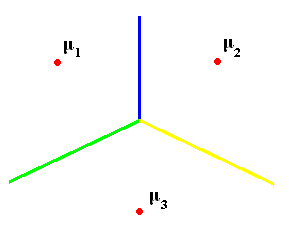
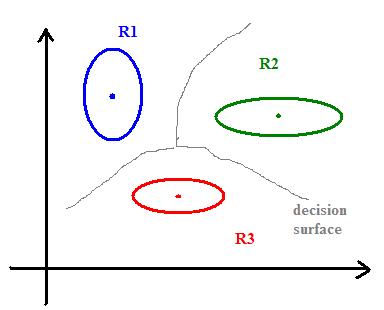
To separate several classes, we can draw the "skeleton" (Blum) of shape defined by mean vectors:
skeleton= set of points whose distance to the set $ \mu_1, ..., \mu_k $ is achieved by at least two different $ \mu_{i}'s $, i.e., we have $ dist(x,set)=min \{dist(x,\mu_i)\} $
and want $ \exists i_1 \neq i_2 $ such that $ dist(x,set)=dist(x,\mu_i1) =dist(x,\mu_i2) $
The skeleton is a decision boundary defining regions (chambers) $ R_i $ where we should decide $ w_i $.
What is the equation of these hyperplanes?
Recall the hyperplane equation: $ \{ \vec{x} | \vec{n} \cdot \vec{x} = const \} $
$ \vec{n} $ is a normal vector to the plane. Because if $ \vec{x_1} $ and $ \vec{x_2} $ are in this plane,
$ \Longrightarrow \vec{n} \cdot \vec{x_1} = const, \vec{n} \cdot \vec{x_2} = const $
$ \Longrightarrow \vec{n} \cdot (\vec{x_1} - \vec{x_2}) = const - const = 0 $
$ \therefore \vec{n} \bot ( \vec{x_1} - \vec{x_2}) $
Any linear structure can be written as
$ \sum_{i=1}^{n} c_i x_i + const = 0 $
Ex. of planes in $ \Re^{2} $
Example: for two classes $ w_1 $, $ w_2 $ hyperplane is defined by
$ \{ \vec{x} | g_1(\vec{x}) - g_2(\vec{x}) = 0 \} $
where, $ g_i(\vec{x})=-\frac{1}{2\sigma^2} \|\vec{x}-\mu_i\|_{L_2}^2+ \ln P(w_i) $
$ -\frac{1}{2\sigma^2} ((\vec{x}-\mu_i)^{\top}(\vec{x}-\mu_i)) + \ln P(w_i) $
$ -\frac{1}{2\sigma^2} (\vec{x}^{\top}\vec{x} - \vec{x}^{\top}\mu_i -\mu_i^{\top}\vec{x} + \mu_i^{\top}\mu_i ) + \ln P(w_i) $
but $ \vec{x}^{\top}\vec{\mu_i} $ is scalar $ \Longrightarrow \left( \vec{x}^{\top} \vec{\mu_i}\right)^{\top} = \vec{\mu_i}^{\top}\vec{x} = \vec{x}^{\top}\vec{\mu_i} $
$ \Longrightarrow g_i(\vec{x}) = -\frac{1}{2\sigma^2} \|\vec{x}\|^2 + \frac{1}{\sigma^2} \vec{x} \cdot \vec{\mu_i} - \frac{\mu_i^{\top}\mu_i}{2\sigma^2} + \ln P(w_i) $
First term is independent of $ i $, therefore we can remove first term from $ g_i\left( \vec{x}\right) $
$ \Longrightarrow g_i(\vec{x}) = \frac{1}{\sigma^2} \vec{x} \cdot \vec{\mu_i} - \frac{\vec{\mu_i} \cdot \vec{\mu_i}}{2 \sigma^2} + \ln P(w_i) $
which is a degree one polynomial in $ \vec{x} $.
A classifier that uses a linear discriminant function is called "linear machine".
The hyperplane between two classes is defined by
$ g_1(\vec{x}) - g_2(\vec{x}) = 0 $
$ \Leftrightarrow \frac{1}{\sigma^2} \vec{x}^{\top}\mu_1 - \frac{\mu_1^{\top}\mu_1}{2\sigma^2} + \ln P(w_1) $
$ - \frac{1}{\sigma^2} \vec{x}^{\top}\mu_2 + \frac{\mu_2^{\top}\mu_2}{2\sigma^2} - \ln P(w_2) = 0 $
$ \Leftrightarrow \frac{1}{\sigma^2} \vec{x} \cdot (\vec{\mu_1} - \vec{\mu_2}) =\frac{ \|\vec{\mu_1} \|^2}{2\sigma^2} - \frac{ \|\vec{\mu_2} \|^2}{2\sigma^2} + \ln P(w_2) -\ln P(w_1) $
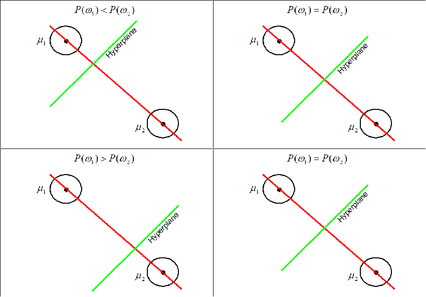
Case 1: When $ P(w_1)=P(w_2) $
The hyperplane (black line) in this case goes through the middle line of the vector (gray line).
Case 2: $ \Sigma_i = \Sigma $ for all i's:
Recall: we can take $ g_i(\vec{x}) = -\frac{1}{2}\left( \vec{x}-\vec{\mu_i} \right)^{\top} \Sigma^{-1}\left(\vec{x}-\vec{\mu_i}\right) - \frac{n}{2}\ln 2\pi - \frac{1}{2} \ln |\Sigma| + \ln P(w_i) $
but $ \Sigma_i = \Sigma, - \frac{1}{2} \ln{2\pi} $ are independent of $ i $
Therefore, we remove these terms from $ g_i(\vec{x}) $, then new $ g_i(\vec{x}) $ will look like
$ \Longrightarrow g_i\left( \vec{x} \right) = - \frac{1}{2} \left( \vec{x} - \vec{\mu_i} \right)^{\top} \Sigma^{-1} \left( \vec{x} - \vec{\mu_i} \right) + \ln{P(w_i)} $
So, if all $ P\left( w_i \right) $'s are the same, assign $ \vec{x} $ to the class with the "nearest" mean.
Rewriting $ g_i(\vec{x}) $,
$ g_i(\vec{x}) = - \frac{1}{2} ( \vec{x}^{\top} \Sigma^{-1}\vec{x} - 2 \vec{\mu_i}^{\top} \Sigma^{-1}\vec{x} + \vec{\mu_i}^{\top}\Sigma^{-1}\vec{\mu_i}) + \ln{P(w_i)} $
Here we know that $ \vec{x}^{\top} \Sigma^{-1}\vec{x} $ is independent of $ i $, therefore we can remove this term from $ g_i(\vec{x}) $
$ \Longrightarrow g_i(\vec{x}) = \vec{\mu_i}^{\top} \Sigma^{-1}\vec{x} - \frac{1}{2} \vec{\mu_i}^{\top}\Sigma^{-1}\vec{\mu_i} + \ln{P(w_i)} $
Again this is a linear function of $ \vec{x} $
The equation of the hyperplane: $ (\vec{\mu_1}-\vec{\mu_2})^{\top}\Sigma^{-1}\vec{x} = \frac{1}{2} \vec{\mu_2}^{\top}\Sigma^{-1}\vec{\mu_2} - \frac{1}{2}\vec{\mu_1}^{\top}\Sigma^{-1}\vec{\mu_1} + \ln P(w_1) - \ln P(w_2) $
In sum, whatever the covariance structures are, as long as they are the same for all classes, the final discriminant functions would be linear (square terms dropped).
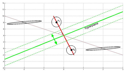
Below, you see an illustration of this case. If you have ellipses that have the same length and direction of the principal axis, you can modify them simultaneously to use Case 1.
The hyperplane (green line) is perpendicular to the red line conecting the two means. It moves along the red line depending on the value of $ P(w_1) $ and $ P(w_2) $. If $ P(w_1)=P(w_2) $ the hyperplane is located on the middle of the distance between the means.
Here's an animated version of the above figure:
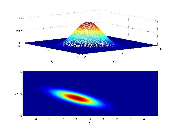
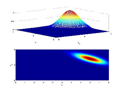
Another visualization for Case 2 is as follows: Consider class 1 which provides a multivariate Gaussian density on a 2D feature vector, when conditioned on that class.
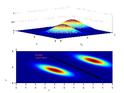
Now consider class 2 with a similar Gaussian conditional density, but with different mean
If the priors for each class are the same (i.e. 0.5), we have that the decision hypersurface cuts directly between the two means, with a direction parallel to the eliptical shape of the modes of the Gaussian densities shaped by their (identical) covariance matrices.
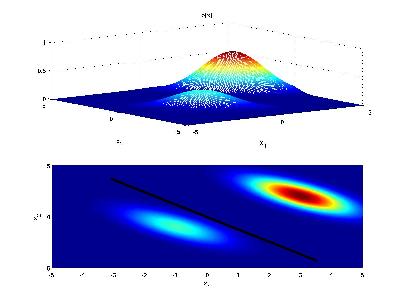
Now if the priors for each class are unequal, we have that the decision hypersurface cuts between the two means with a direction as before, but now will be located further from the more likely class. This biases the estimator in favor of the more likely class.
A video to visualize the decision hypersurface with changes to the Gaussian parameters is shown on the [Bayes Decision Rule] page.
Case 3: When $ \Sigma_i^{-1} $ is arbitrary
We can take
$ g_i(\vec{x}) = - \frac{1}{2} ( \vec{x} - \vec{\mu_i})^{\top}\Sigma_i^{-1}(\vec{x}-\vec{\mu_i})-\frac{1}{2} \ln \|\Sigma_i\|+ \ln P(w_i) $
the decision surface between $ w_1 $ and $ w_2 $:
is a degree 2 polynom in $ \vec{x} $
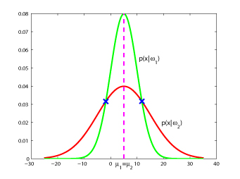
Note: decision boundaries must not be connected if $ P(w_1)=P(w_2) $ decision boundary has two disconnected points.
Class =w1, when -5<x<15
Class=w2, when x<-5 or x>15
For difference cases and their figures, refer to page 42 and 43 of DHS.

