Difference between revisions of "Lecture 5 - Discriminant Functions OldKiwi" - Rhea

Revision as of 14:51, 13 June 2008

LECTURE THEME : - Discriminant Functions

Discriminant Functions: one way of representing classifiers

Given the classes $ \omega_1, \cdots, \omega_k $

The discriminant functions $ g_1(x),\ldots, g_K(x) $ such that $ g_i(x) $ n-dim S space $ \rightarrow \Re $

which are used to make decisions as follows:

decide $ \omega_i $ if $ g_i(x) \ge g_j(x), \forall j $

Note that many different choices of $ g_i(x) $ will yield the same decision rule, because we are interested in the order of values of $ g_i(x) $ for each x, and not their exact values.

For example: $ g_i(x) \rightarrow 2(g_i(x)) $ or $ g_i(x) \rightarrow ln(g_i(x)) $

In other words, we can take $ g_i(x) \rightarrow f(g_i(x)) $ for any monotonically increasing function f.

Relation to Bayes Rule

e.g. We can take $ g_i(\mathbf(x)) = P(\omega_i|\mathbf(x)) $

then $ g_i(\mathbf(x)) > g_j(\mathbf(x)), \forall j \neq i $

$ \Longleftrightarrow P(w_i|\mathbf(X)) > P(w_j|\mathbf(X)), \forall j \neq i $

OR we can take

$ g_i(\mathbf(x)) = p(\mathbf(x)|\omega_i)P(\omega_i) $

then $ g_i(\mathbf(x)) > g_j(\mathbf(x)), \forall j \neq i $

$ \Longleftrightarrow g_i(\mathbf(x)) = ln(p(\mathbf(x)|\omega_i)P(\omega_i)) = ln(p(\mathbf(x)|\omega_i))+ln(P(\omega_i) $

OR we can take

$ g_i(\mathbf(x)) = ln(p(\mathbf(x)|\omega_i)P(\omega_i)) = ln(p(\mathbf(x)|\omega_i))+ln(P(\omega_i) $

We can take any $ g_i $ as long as they have the same ordering in value as specified by Bayes rule.

Some useful links:

- Bayes Rule in notes: https://engineering.purdue.edu/people/mireille.boutin.1/ECE301kiwi/Lecture4

- Bayesian Inference: http://en.wikipedia.org/wiki/Bayesian_inference

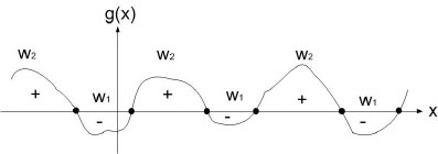
Relational Decision Boundary

Ex : take two classes $ \omega_1 $ and $ \omega_2 $

$ g(\vec x)=g_1(\vec x)-g_2(\vec x) $

decide $ \omega_1 $ when $ g(\vec x)>0 $

and $ \omega_2 $ when $ g(\vec x)<0 $

when $ g(\vec x) = 0 $, you are at the decision boundary ( = hyperplane)

$ \lbrace \vec x | \vec x \;\;s.t \;\;g(\vec x)=0\rbrace $ is a hypersurface in your feature space i.e a structure of co-dimension one less dimension than space in which $ \vec x $ lies

Figure 1

Discriminant function for the Normal Density

Suppose we assume that the distribution of the feature vectors is such that the density function p(X|w) is normal for all i.

Eg: Length of hair among men is a normal random variable. Same for hairlength in women. Now we have:

is the Mahalanobis Distance Squared from X from mui

Figure 2

For simplicity, add n/2ln(2pi) to all gi's. Then we get:

Prior Term:

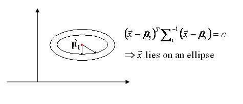
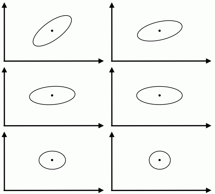
If classes are equally likely, then we can get rid of the first term. If the Distribution Matrix is the same, then the second term goes off. Special case 1: "Spherical clusters" in n-dimensional space. Equidistant points lie on a circle around the average values. 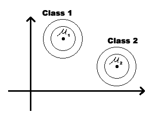Figure 3

Final Note on Lecture 5:

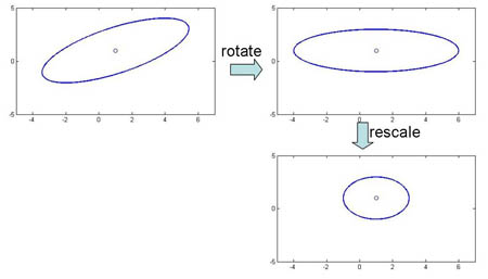
We could modify the coordinates of a class feature vector (as shown on the figure below) to take advantage of Special Case 1. But you should be aware that, in general, this can not be done for all classes simultaneously.

Figure 4

Figure 5