(New page: ==Buggy Code== F0 =13; T0 =1/F0; Ts = 0.07; t = 0:Ts:13*T0; x = real(exp(j*(2*pi*F0*t-pi/2))); plot(t,x) The above MATLAB code is supposed to output 13 cycles of a 13 Hz sine wave. How...) |
(→Buggy Code) |
||
| Line 1: | Line 1: | ||
==Buggy Code== | ==Buggy Code== | ||
| − | F0 =13; | + | F0 =13; |
| − | T0 =1/F0; | + | T0 =1/F0; |
| − | Ts = 0.07; | + | Ts = 0.07; |
| − | t = 0:Ts:13*T0; | + | t = 0:Ts:13*T0; |
| − | x = real(exp(j*(2*pi*F0*t-pi/2))); | + | x = real(exp(j*(2*pi*F0*t-pi/2))); |
| − | plot(t,x) | + | plot(t,x) |
The above MATLAB code is supposed to output 13 cycles of a 13 Hz sine wave. However, it instead outputs this: | The above MATLAB code is supposed to output 13 cycles of a 13 Hz sine wave. However, it instead outputs this: | ||
| Line 23: | Line 23: | ||
F0 =13; | F0 =13; | ||
| − | |||
T0 =1/F0; | T0 =1/F0; | ||
| − | |||
Ts = 0.005; | Ts = 0.005; | ||
| − | |||
t = 0:Ts:13*T0; | t = 0:Ts:13*T0; | ||
| − | |||
x = real(exp(j*(2*pi*F0*t-pi/2))); | x = real(exp(j*(2*pi*F0*t-pi/2))); | ||
| − | |||
plot(t,x) | plot(t,x) | ||
Latest revision as of 11:10, 12 September 2008
Buggy Code
F0 =13;
T0 =1/F0;
Ts = 0.07;
t  = 0:Ts:13*T0;
x = real(exp(j*(2*pi*F0*t-pi/2)));
plot(t,x)
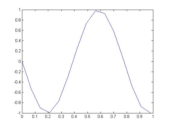
The above MATLAB code is supposed to output 13 cycles of a 13 Hz sine wave. However, it instead outputs this:
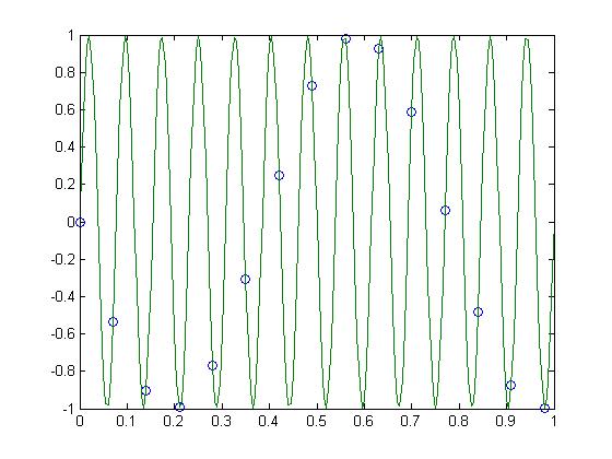
The problem is with the sampling rate Ts. Ts is .07, and the frequency of the sine wave is 13. 1/13 is .769. A sampling rate so close to the inverse of the frequency is not going to yield enough data points to give an accurate graph. Taking a much smaller sampling rate of .005 will give a better graph of the data. Below is the graph with a sampling rate of .005, overlaid with the original graph shown by circles.
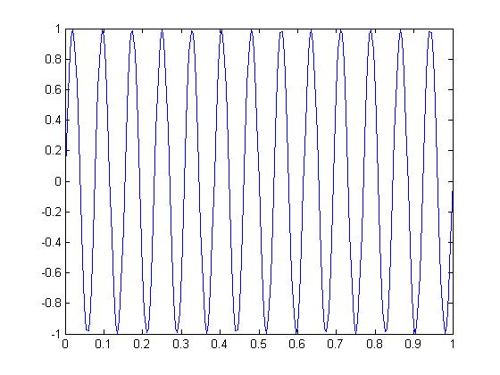
And here is the proper wave output by itself:
Here is the code to output the proper wave:
F0 =13;
T0 =1/F0;
Ts = 0.005;
t  = 0:Ts:13*T0;
x = real(exp(j*(2*pi*F0*t-pi/2)));
plot(t,x)


