(→Part 2) |
|||
| Line 6: | Line 6: | ||
Note: The code used to make this plot is a modified version of Ben Horst's. | Note: The code used to make this plot is a modified version of Ben Horst's. | ||
| + | |||
| + | <pre> | ||
| + | delta = .0001; | ||
| + | period = 10; | ||
| + | repetitions = 5; | ||
| + | |||
| + | t = [delta:delta:period]; | ||
| + | a = t; | ||
| + | c = []; | ||
| + | for i=1:repetitions | ||
| + | c = [c,a]; | ||
| + | end | ||
| + | t = [delta:delta:period*repetitions]; | ||
| + | plot(t,c) | ||
| + | </pre> | ||
Revision as of 09:59, 12 September 2008
Part 2
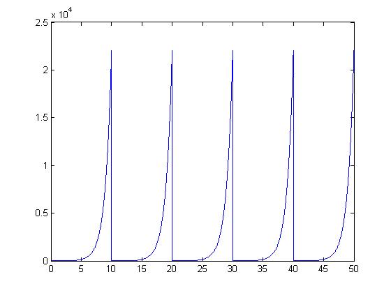
I choose the function of $ e^t $ from the one posted under Hw 1.4 David Hartmann. I use period of 10 to create this signal to be a periodic one. The plot is shown below:
Note: The code used to make this plot is a modified version of Ben Horst's.
delta = .0001;
period = 10;
repetitions = 5;

t = [delta:delta:period];
a = t;
c = [];
for i=1:repetitions
   c = [c,a];
end
t = [delta:delta:period*repetitions];
plot(t,c)


