| Line 3: | Line 3: | ||
=Python Demonstration= | =Python Demonstration= | ||
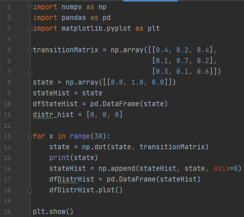
| − | We will be using Python to demonstrate Markov chains. The following program was taken from [https://towardsdatascience.com/markov-chain-analysis-and-simulation-using-python-4507cee0b06e this article] and modified to fit our example. | + | We will be using Python to demonstrate Markov chains. The following program was taken from [https://towardsdatascience.com/markov-chain-analysis-and-simulation-using-python-4507cee0b06e this article] and modified to fit our example. This is not a computer science presentation, but to help the reader understand what is happening, here is a brief explanation of the program (refer to the line numbers on the left of the images): |
<center>[[File:Pythondemo1.png|500px|thumbnail]]</center> | <center>[[File:Pythondemo1.png|500px|thumbnail]]</center> | ||
| − | + | Lines 1-3: Importing packages that we will be using in this program. ''NumPy'' is used to work with matrices and lists, and ''pandas'' is used to manipulate data structures. ''Matplotlib'' is used to display a graph to the user. | |
| − | + | Line 5-7: We create a variable ''transitionMatrix'' that holds the transition matrix values from our example. | |
| − | + | Line 8-11: The list variable state is created and resembles the state demonstrated in the above scenario. The following lines are used to create a plot of the current data. Note that we create another variable ''stateHist'' that currently holds the same values as state. This will be important later on. | |
| − | + | Lines 13-18: This is the for loop where we iterate through the Markov chain. The first line states that we will be looping through the code in lines 14-18 as long as the variable x is less than 30. In simpler terms, this means that the code will be repeated 30 times (because ''x'' starts at a value of 0). | |
| + | Then, we take the dot product of state and ''transitionMatrix'' using the ''np.dot'' function and store the new dot product in our state variable. The state variable here is the same as the one in line 8, but it is now being updated to hold the dot product. | ||
| + | Afterwards, we print the new dot product to the console for the user to see and append the dot product to ''stateHist'' so that it now holds our original state and the updated state. Finally, the last two lines add the new data to the graph. | ||
| − | + | Line 20: This uses the ''matplotlib'' package we imported to show us the plot we have created. | |
| + | <center>[[File:Pythondemo2.png|900px|thumbnail]]</center> | ||
| + | |||
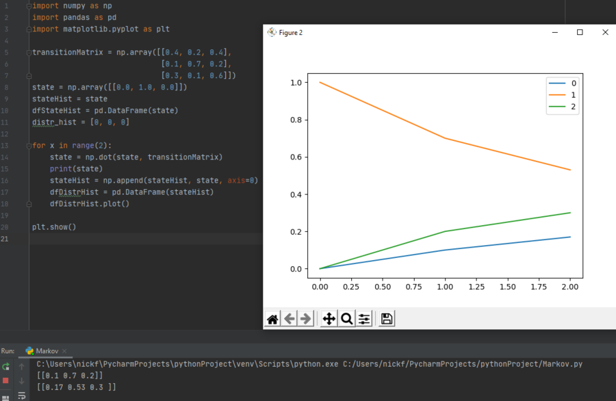
| + | To verify that the program is accurate, we set the for loop to run only twice (as seen in line 13, where ''x'' now must be less than 2 in order to continue iteration). Pictured above is the plot we obtain in those two steps through the Markov chain, and at the very bottom we have the actual dot product calculations printed to the console, which we can verify are consistent with our own calculations. | ||
| + | |||
| + | '''NOTE:''' In the plot, the yellow line represents a sunny state, the blue line represents a rainy state, and the green line represents a cloudy state. | ||
| + | |||
| + | <center>[[File:Pythondemo3.png|900px|thumbnail]]</center> | ||
| + | |||
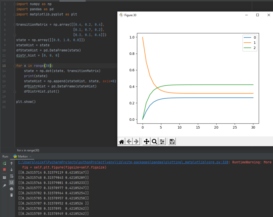
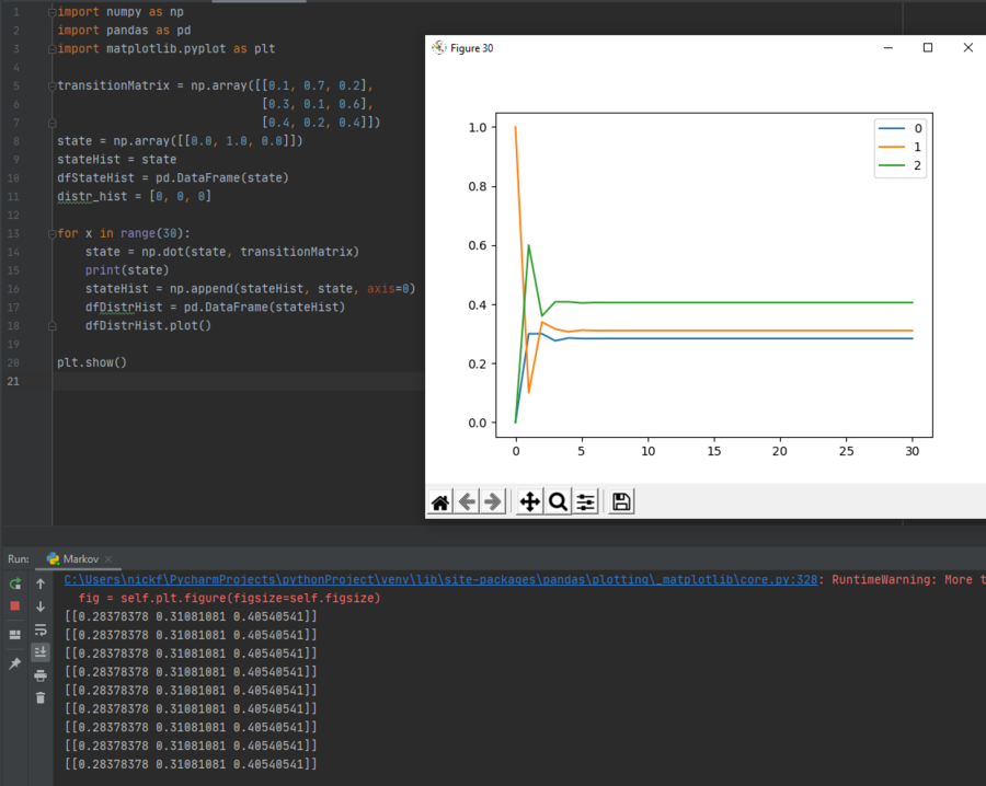
| + | Here, we have set the for loop back to continue iteration as long as x is less than 30, and we see that over time, the probabilities of each state will stabilize. This holds true for all Markov chains, no matter the transition matrix. For example, if the transition matrix rows were to be scrambled, we can see that although the probability of each state occurring does change, the probabilities will still stabilize, as shown below: | ||
| + | |||
| + | <center>[[File:Pythondemo4.png|900px|thumbnail]]</center> | ||
| + | |||
| + | As another verification, we can change the state vector. If instead of the first day being sunny it was rainy, we can see that the probabilities once again stabilize: | ||
| + | |||
| + | <center>[[File:Pythondemo5.png|900px|thumbnail]]</center> | ||
| + | |||
| + | Finally, if we are to attempt to use an impossible state vector, although the probabilities do stabilize, they do not add up to one, which confirms that both the solved probabilities and the state vector are invalid. Notice the state vector values in the terminal window at the very bottom. They are <math>[0.2631579, 0.31578947, 0.42105263]</math>. These values will be used later in this paper. | ||
| + | |||
| + | <center>[[File:Pythondemo6.png|900px|thumbnail]]</center> | ||
| + | |||
| + | Here, the current state vector has been altered so that it now reads <math>[1, 1, 0]</math>, which means that the current day is both rainy and sunny. This results in probabilities that do not add up to one, making them invalid. This makes sense because in the context of our example, there is no possible way for the current state to be both rainy and sunny (this is under the assumption that the weather stays constant for the entire day). | ||
[[ Walther MA271 Fall2020 topic2|Back to Markov Chains]] | [[ Walther MA271 Fall2020 topic2|Back to Markov Chains]] | ||
[[Category:MA271Fall2020Walther]] | [[Category:MA271Fall2020Walther]] | ||
Latest revision as of 23:57, 5 December 2020
Python Demonstration
We will be using Python to demonstrate Markov chains. The following program was taken from this article and modified to fit our example. This is not a computer science presentation, but to help the reader understand what is happening, here is a brief explanation of the program (refer to the line numbers on the left of the images):
Lines 1-3: Importing packages that we will be using in this program. NumPy is used to work with matrices and lists, and pandas is used to manipulate data structures. Matplotlib is used to display a graph to the user.
Line 5-7: We create a variable transitionMatrix that holds the transition matrix values from our example.
Line 8-11: The list variable state is created and resembles the state demonstrated in the above scenario. The following lines are used to create a plot of the current data. Note that we create another variable stateHist that currently holds the same values as state. This will be important later on.
Lines 13-18: This is the for loop where we iterate through the Markov chain. The first line states that we will be looping through the code in lines 14-18 as long as the variable x is less than 30. In simpler terms, this means that the code will be repeated 30 times (because x starts at a value of 0). Then, we take the dot product of state and transitionMatrix using the np.dot function and store the new dot product in our state variable. The state variable here is the same as the one in line 8, but it is now being updated to hold the dot product. Afterwards, we print the new dot product to the console for the user to see and append the dot product to stateHist so that it now holds our original state and the updated state. Finally, the last two lines add the new data to the graph.
Line 20: This uses the matplotlib package we imported to show us the plot we have created.
To verify that the program is accurate, we set the for loop to run only twice (as seen in line 13, where x now must be less than 2 in order to continue iteration). Pictured above is the plot we obtain in those two steps through the Markov chain, and at the very bottom we have the actual dot product calculations printed to the console, which we can verify are consistent with our own calculations.
NOTE: In the plot, the yellow line represents a sunny state, the blue line represents a rainy state, and the green line represents a cloudy state.
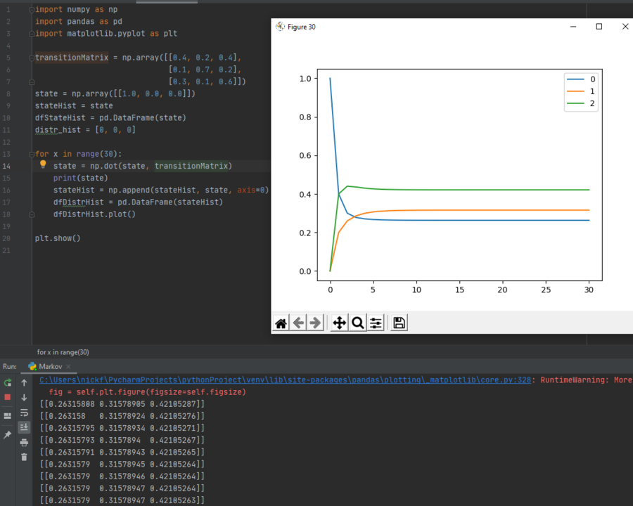
Here, we have set the for loop back to continue iteration as long as x is less than 30, and we see that over time, the probabilities of each state will stabilize. This holds true for all Markov chains, no matter the transition matrix. For example, if the transition matrix rows were to be scrambled, we can see that although the probability of each state occurring does change, the probabilities will still stabilize, as shown below:
As another verification, we can change the state vector. If instead of the first day being sunny it was rainy, we can see that the probabilities once again stabilize:
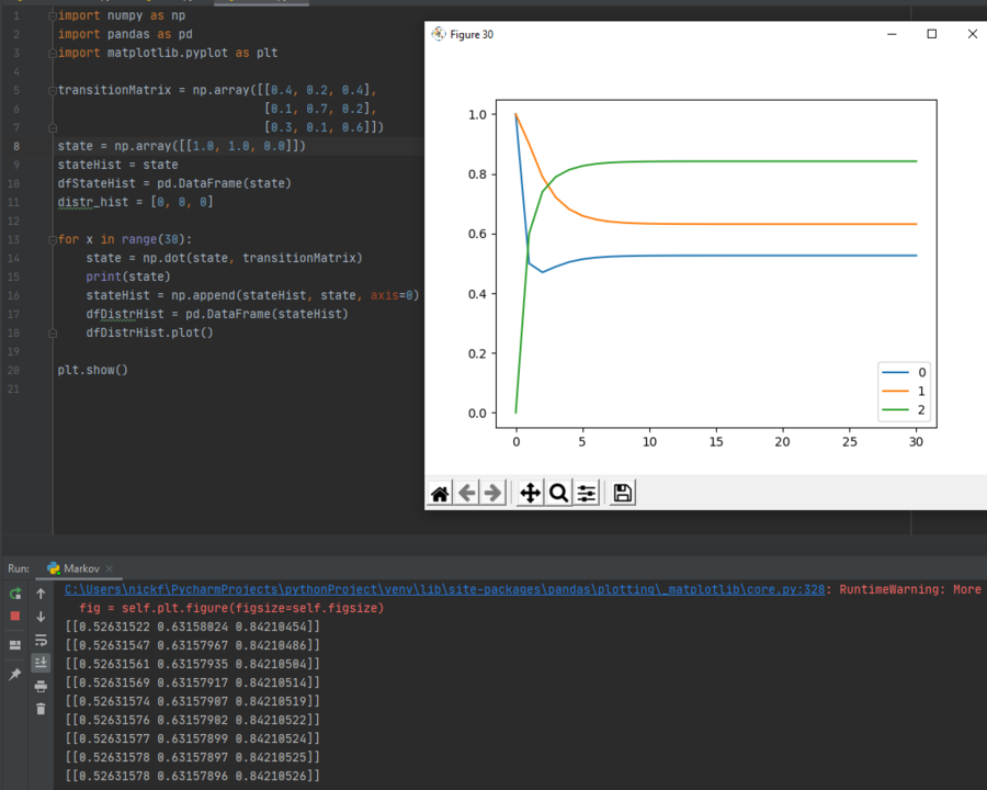
Finally, if we are to attempt to use an impossible state vector, although the probabilities do stabilize, they do not add up to one, which confirms that both the solved probabilities and the state vector are invalid. Notice the state vector values in the terminal window at the very bottom. They are $ [0.2631579, 0.31578947, 0.42105263] $. These values will be used later in this paper.
Here, the current state vector has been altered so that it now reads $ [1, 1, 0] $, which means that the current day is both rainy and sunny. This results in probabilities that do not add up to one, making them invalid. This makes sense because in the context of our example, there is no possible way for the current state to be both rainy and sunny (this is under the assumption that the weather stays constant for the entire day).

