| Line 9: | Line 9: | ||
<br>1.What is a Markov chain?<br>To answer this question, we need to know the definition of a stochastic process, because a Markov Chain is a special type of stochastic process. <br>Definition of a stochastic process:<br> “A sequence of random variables X1, X2,…,Xn is called a stochastic process with discrete time parameter n.” [1] | <br>1.What is a Markov chain?<br>To answer this question, we need to know the definition of a stochastic process, because a Markov Chain is a special type of stochastic process. <br>Definition of a stochastic process:<br> “A sequence of random variables X1, X2,…,Xn is called a stochastic process with discrete time parameter n.” [1] | ||
| − | Explanation: We may think X1, X2,…,Xn as samples of an experiment. In a stochastic process, they represent states of processes. Clearly, X1 is called the initial state | + | Explanation: We may think X1, X2,…,Xn as samples of an experiment. In a stochastic process, they represent states of processes. Clearly, X1 is called the initial state and Xn represents the state at time n. In an introductory probability course, we are familiar with the models when X1,…,Xn are independently identical distributed (iid) random variables. However, note that states do not necessarily have to be independently identically distributed. This note is especially important to eliminate confusion for first time learners in the Markov Chain. |
<br> | <br> | ||
| − | Definition of a Markov | + | Definition of a Markov Chain: <br>A stochastic process is a Markov Chain if, for every time n, the conditional distributions of all Xn+j given X1,…,Xn depend only on Xn instead of X1,…,Xn-1. In the majority or basic cases, we consider j=1. That is, the probability distribution of random variable Xn is determined by the value from the (n-1)th state (Xn-1). This means the distribution of future states depend only on the present state, and has nothing to do with the past states.<br>*Note: In a Markov Chain, the value of present state only determines the “probability distribution of the future state”, it does not determine the exact value of the future states. |
<br> | <br> | ||
| − | A concrete example<br>Let’s consider a person has two choices of | + | A concrete example:<br>Let’s consider a person has two choices of drinks for his breakfast every morning, milk or coffee. We let Xi=1 if the person chooses to drink milk on the i'th morning. Let Xi=2 if the person chooses to drink coffee on the i'th morning. In this case, the sequence of cases (random variables) X1, X2… is a stochastic process with two possible states at each time. To make it be a Markov chain, consider that most people will usually switch rather than drink the same thing every day, and our person prefers milk more than coffee. Thus assume probability of that person choosing milk today given he chose milk yesterday is 0.3. The probability that he chooses coffee given he chose coffee yesterday is 0.2. Then this sequence of states becomes a Markov Chain. <br><br> <br><span class="texhtml">''P''(''X''<sub>''n'' + 1</sub> = 1 | ''X''<sub>''n''</sub> = 1) = 0.3</span>, <span class="texhtml">''P''(''X''<sub>''n'' + 1</sub> = 2 | ''X''<sub>''n''</sub> = 1) = 1 − 0.3 = 0.7</span><br> <br><span class="texhtml">''P''(''X''<sub>''n'' + 1</sub> = 1 | ''X''<sub>''n''</sub> = 2) = 1 − 0.2 = 0.8</span>, <span class="texhtml">''P''(''X''<sub>''n'' + 1</sub> = 2 | ''X''<sub>''n''</sub> = 2) = 0.2</span><br> <br>[[Image:Milk and Coffee.PNG]]<br> What can we do with this?<br> Transition probabilities and Transition Matrix<br>We define P_ij to be the probability that the future state is j given the present state is i.<br><span class="texhtml">''P''(''X''<sub>''n'' + 1</sub> = ''j'' | ''X''<sub>''n''</sub> = ''i'') = ''P''<sub>''i''''j'''''</sub></span>'''''<br>They are called transition distributions. If a Markov Chain’s transition distributions do not depend on n (just like the above example), then we call the Markov Chain has stationary transition distributions.<br>In particular, a Markov Chain with stationary transition distributions can be presented by a Transition Matrix. For instance, the transition Matrix for the above Example is:<br> <br><math>\begin{pmatrix} |
0.3 & 0.7 \\ | 0.3 & 0.7 \\ | ||
0.8 & 0.2 | 0.8 & 0.2 | ||
Revision as of 10:41, 25 March 2014
What is a Markov chain/process? What can you do with it? And why are lots of people talking about them?
Back to MA375 Spring 2014
Tianyi Zhang: zhan1035@purdue.edu ;
Sui Fang: fang52@purdue.edu ;
Christopher Peralta: cperalta@purdue.edu;
Lei Zhong: zhong9@purdue.edu ;
Nathan Accornero: naccorne@purdue.edu
Outline of the Project:
A) What is a Markov Chain?
-Stochastic process
-Definition of Markov Chain
-Concrete examples and several properties
B) What can we do with it?
-Transition Probabilities and Transition Matrix
-Computation with Transition Matrix
-Matrix limits and Markov Chains
C) Why is a Markov Chain useful?
-Applications in Real Life with examples and computation
1.What is a Markov chain?
To answer this question, we need to know the definition of a stochastic process, because a Markov Chain is a special type of stochastic process.
Definition of a stochastic process:
“A sequence of random variables X1, X2,…,Xn is called a stochastic process with discrete time parameter n.” [1]
Explanation: We may think X1, X2,…,Xn as samples of an experiment. In a stochastic process, they represent states of processes. Clearly, X1 is called the initial state and Xn represents the state at time n. In an introductory probability course, we are familiar with the models when X1,…,Xn are independently identical distributed (iid) random variables. However, note that states do not necessarily have to be independently identically distributed. This note is especially important to eliminate confusion for first time learners in the Markov Chain.
Definition of a Markov Chain:
A stochastic process is a Markov Chain if, for every time n, the conditional distributions of all Xn+j given X1,…,Xn depend only on Xn instead of X1,…,Xn-1. In the majority or basic cases, we consider j=1. That is, the probability distribution of random variable Xn is determined by the value from the (n-1)th state (Xn-1). This means the distribution of future states depend only on the present state, and has nothing to do with the past states.
*Note: In a Markov Chain, the value of present state only determines the “probability distribution of the future state”, it does not determine the exact value of the future states.
A concrete example:
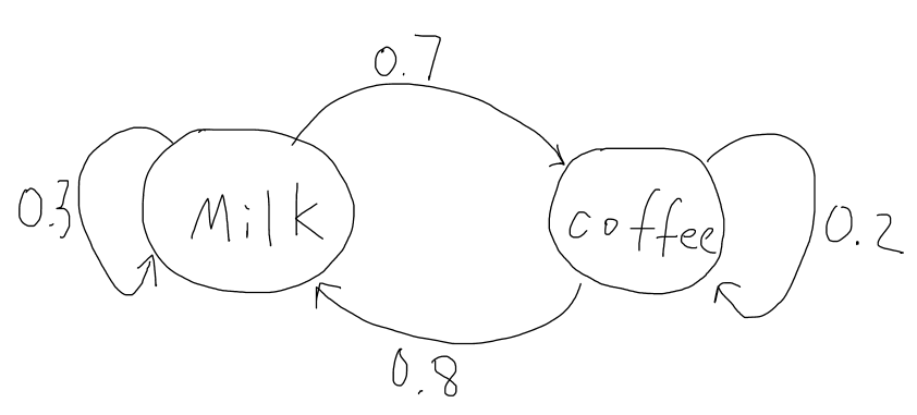
Let’s consider a person has two choices of drinks for his breakfast every morning, milk or coffee. We let Xi=1 if the person chooses to drink milk on the i'th morning. Let Xi=2 if the person chooses to drink coffee on the i'th morning. In this case, the sequence of cases (random variables) X1, X2… is a stochastic process with two possible states at each time. To make it be a Markov chain, consider that most people will usually switch rather than drink the same thing every day, and our person prefers milk more than coffee. Thus assume probability of that person choosing milk today given he chose milk yesterday is 0.3. The probability that he chooses coffee given he chose coffee yesterday is 0.2. Then this sequence of states becomes a Markov Chain.
P(Xn + 1 = 1 | Xn = 1) = 0.3, P(Xn + 1 = 2 | Xn = 1) = 1 − 0.3 = 0.7
P(Xn + 1 = 1 | Xn = 2) = 1 − 0.2 = 0.8, P(Xn + 1 = 2 | Xn = 2) = 0.2
What can we do with this?
Transition probabilities and Transition Matrix
We define P_ij to be the probability that the future state is j given the present state is i.
P(Xn + 1 = j | Xn = i) = Pi''j
They are called transition distributions. If a Markov Chain’s transition distributions do not depend on n (just like the above example), then we call the Markov Chain has stationary transition distributions.
In particular, a Markov Chain with stationary transition distributions can be presented by a Transition Matrix. For instance, the transition Matrix for the above Example is:
$ \begin{pmatrix} 0.3 & 0.7 \\ 0.8 & 0.2 \end{pmatrix} $
More Generally:$ P=\begin{bmatrix} P_{11} & \cdots & P_{1k} \\ \vdots & \ddots & \vdots \\ P_{k1} & \cdots & P_{kk} \end{bmatrix} $
General Rule for nth state distribution:$ x_n=x_{n-1}P $
Important Notes:
$ P_{ij} $ in the above matrix represents $ P(X_{n+1}=j|X_n=i) $, this turns out the result that the sum of every entries in each row is 1 (This follows the same notation as my probability textbook and most professional articles I have searched in the electronic library). However, in some textbooks (for example, my linear algebra textbook) and resources I found on the Internet, $ P_{ij} $ in the Matrix = $ P(X_{n+1}=i|X_n=j) $, this means the sum of every entries in each column is 1. To avoid confusion, we are going to follow the first notation style in this note.
The transition matrix makes computation in a Markov Chain easier. In the above breakfast example (it has stationary transition probability), if we are given that person drunk milk at time n,$ X_n=1 $, we can determine the probability distribution of $ X_{n+3} $. The initial state distribution can be written as a row vector : $ \begin{pmatrix}1 & 0\end{pmatrix} $
$ x_{n+3}=x_{n+2}P=(x_{n+1}P)P=((x_nP)P)P=x_nP^3=\begin{pmatrix}1 & 0\end{pmatrix} \begin{pmatrix} 0.3 & 0.7 \\ 0.8 & 0.2 \end{pmatrix}^3 $
$ x_{n+3}=\begin{pmatrix}0.475 & 0.525\end{pmatrix} $
This means given the person drunk milk today, three days later, he has probability 0.475 to drink milk and 0.525 to drink coffee.
- Matrix Limits and Markov Chain
In the Linear Algebra courses (MA351 and MA353 in Purdue University), we know that a diagonalizable Matrix A can be represented in a form $ A=QDQ^{-1} $.
Where $ D=\begin{bmatrix} r_{1} & \cdots & 0 \\ \vdots & \ddots & \vdots \\ 0 & \cdots & r_n \end{bmatrix} $, where $ r_1...r_n $ are eigenvalues of the matrix A, and Q are has columns corresponding to the eigenvectors.
$ A^n=QDQ^{-1}QDQ^{-1}...QDQ^{-1}=QD^nQ^{-1}; \lim_{n \to \infty}A^n=\lim_{n \to \infty}(QD^nQ^{-1}) $.
Since D is a diagonal matrix, it’s very easy to compute its powers. In the above breakfast example, we are able to compute the matrix limits.
$ P=\begin{pmatrix} 0.3 & 0.7 \\ 0.8 & 0.2 \end{pmatrix} $;
The Characteristic Polynomial for P is:
$ (0.3-r)(0.2-r)-0.8*0.7=0; r_1=1; r_2=-0.5; Thus,D=\begin{pmatrix} 1 & 0 \\ 0 & -0.5 \end{pmatrix} $
Solving the linear systems, eigenvectors for P are:
$ \begin{pmatrix} 1 \\ 1 \end{pmatrix} and \begin{pmatrix} 7 \\ -8 \end{pmatrix}; Thus, Q=\begin{pmatrix} 1 & 7 \\ 1 & -8 \end{pmatrix} $;
$ \lim_{n \to \infty}P^n=\lim_{n \to \infty}(QD^nQ^{-1})=\lim_{n \to \infty}\begin{pmatrix} 1 & 7 \\ 1 & -8 \end{pmatrix} \begin{pmatrix} 1 & 0 \\ 0 & -0.5 \end{pmatrix}^n \begin{pmatrix} 1 & 7 \\ 1 & -8 \end{pmatrix}^{-1} $
$ =\lim_{n \to \infty}\begin{pmatrix} (8+7(-0.5)^n)/15 & 7/15 \\ (8-8(-0.5)^n)/15 &(7-8(-0.5)^n)/15 \end{pmatrix}= \begin{pmatrix} 8/15 & 7/15 \\ 8/15 & 7/15 \end{pmatrix} $
We put the initial condition into the equation:
$ \begin{pmatrix} 1 & 0 \end{pmatrix}\begin{pmatrix} 8/15 & 7/15 \\ 8/15 & 7/15 \end{pmatrix}=\begin{pmatrix} 8/15 & 7/15 \end{pmatrix} $
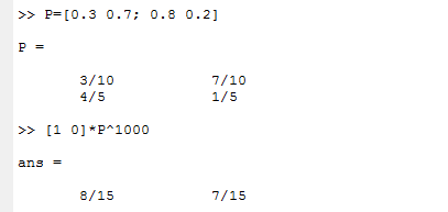
In fact, we will always get $ \begin{pmatrix} 8/15 & 7/15 \end{pmatrix} $ whatever he drinks milk or coffee in the first day. This indicates that in a long time period, he will drink milk in 8/15 of days, and drink coffee in 7/15 of days.
Use MatLab to verify our result, just use n=1000:
3. Why are lots if people talking about Markov Chain?
- Applications of Markov Chain in Science and Real Life
Markov Chains have lots of applications in the scientific research, because many cases can be approximately modeled as a Markov Chain. In economics and finance, Markov Chains can help investors to predict the volatility of asset returns. In biology, Markov chains can be used in population genetics research. In the simplest case, Markov chains are used in weather predictions.
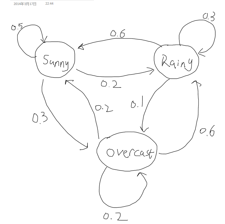
We now construct a very simple sample of weather prediction. Assume a city has 3 weather states: Sunny, Rainy and Overcast. This corresponds to the states space S= {0,1,2}. Suppose that the probability distribution of the next day only depends on the weather state of today (This is relatively reasonable in real cases), and given that:
$ P(X_{n+1}=Sunny|X_n=Sunny)=0.5 $;
$ P(X_{n+1}=Rainy|X_n=Sunny)=0.2 $;
$ P(X_{n+1}=Overcast|X_n=Sunny)=1-0.5-0.2=0.3 $;
$ P(X_{n+1}=Sunny|X_n=Rainy)=0.6 $;
$ P(X_{n+1}=Rainy|X_n=Rainy)=0.3 $;
$ P(X_{n+1}=Overcast|X_n=Rainy)=1-0.6-0.3=0.1 $;
$ P(X_{n+1}=Sunny|X_n=Overcast)=0.2 $;
$ P(X_{n+1}=Rainy|X_n=Overcast)=0.6 $;
$ P(X_{n+1}=Overcast|X_n=Overcast)=1-0.2-0.6=0.2 $;
Transition Matrix P for this Model:
$ \begin{pmatrix} 0.5 & 0.2 & 0.3 \\ 0.6 & 0.3 & 0.1 \\ 0.2 & 0.6 & 0.2 \\ \end{pmatrix} $
Suppose we know the weather is overcast this Monday (Today), then we can determine the probability distribution of weathers in next several days (like Weather forecasting on TV). For instance, on Wednesday:
$ x_{n+2}=x_{n}P^2=\begin{pmatrix} 0 & 0 & 1 \end{pmatrix} \begin{pmatrix} 0.5 & 0.2 & 0.3 \\ 0.6 & 0.3 & 0.1 \\ 0.2 & 0.6 & 0.2 \\ \end{pmatrix} \begin{pmatrix} 0.5 & 0.2 & 0.3 \\ 0.6 & 0.3 & 0.1 \\ 0.2 & 0.6 & 0.2 \\ \end{pmatrix} =\begin{pmatrix} 0.5 & 0.34 & 0.16 \end{pmatrix} $
This means on Wednesday, probability is 0.5 for sunny, 0.34 for rainy and 0.16 for overcast given that Monday is overcast.
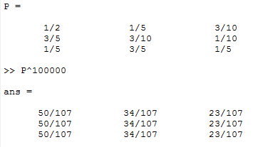
We can also use matrix limits to determine the long-term probability following the procedure in Part II. Since it’s a little bit complicated to diagonalize 3*3 matrix by hand, especially for matrix with complex eigenvalues and eigenvectors, we use Matlab instead:
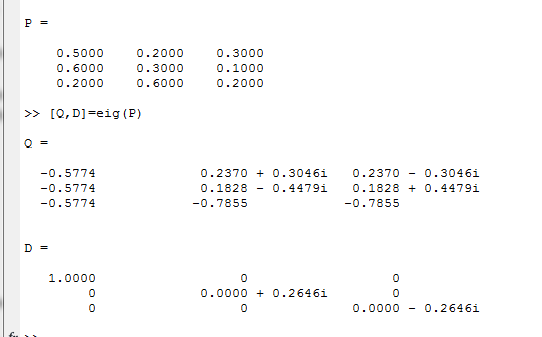
$ \lim_{n \to \infty}P^n=\lim_{n \to \infty}(QD^nQ^{-1})=\begin{pmatrix} 50/107 & 34/107 & 23/107 \\ 50/107 & 34/107 & 23/107 \\ 50/107 & 34/107 & 23/107 \\ \end{pmatrix} $
Therefore, for a single day randomly picked up from the calendar, this city has the probability 50/107 of sunny weather, 34/107 for rainy weather and 23/107 for overcast weather.
Verify the result by Matlab, take n=10000:
The weather model made up by me is just a very simple example in real application related to Markov Chain, many other models, such as PageRank in Google, are also using the Markov Chain. Yet it’s too complicated somehow to show on this Webpage. Besides, we are also not able to talk about some further topics of Markov Chain, such as Hidden Markov Model or Markov Chain in continuous time.
This project was originally conducted by Office Word, a link for the PDF file (already uploaded to this site)
can be found
References and Theorems & knowledge Sources:
- Morris H. Degroot, Mark J. Schervish, Probability and Statistics, 4th edition
- Michael J. Evans, Jeffery S. Rosenthal, Probability and Statistics: The Science of Uncertainty, 2nd edition
- Stephen H. Friedberg, Arnold J. Insel, Linear Algebra, 4th edition

