| Line 19: | Line 19: | ||
<math> \rho (X,Y) = \frac{cov(X,Y)}{ \sqrt{var(X)var(Y)} } </math> | <math> \rho (X,Y) = \frac{cov(X,Y)}{ \sqrt{var(X)var(Y)} } </math> | ||
| − | Covariance is defined as: <math> C_{s}(n1, n2) = E(X-E[X])(Y-E[Y]))</math>[https://engineering.purdue.edu/~ipollak/ece302/SPRING12/notes/19_GeneralRVs-4_Multiple_RVs.pdf] | + | Covariance is defined as: <math> C_{s}(n1, n2) = E(X-E[X])(Y-E[Y]))</math> [https://engineering.purdue.edu/~ipollak/ece302/SPRING12/notes/19_GeneralRVs-4_Multiple_RVs.pdf] |
| − | + | ||
| − | If X and Y are independent of each other, that means they are uncorrelated with each other, or cov(X,Y) = 0. However, if X and Y are uncorrelated, that does not mean they are independent of each other. 1, -1, and 0 are the three extreme points <math>p\rho X,Y)</math> can represent. 1 represents that X and Y are linearly dependent of each other. In other words, Y-E[Y] is a positive multiple of X-E[X]. -1 represents that X and Y are inversely dependent of each other. In other words, Y-E[Y] is a negative multiple of X-E[X]. [ | + | Correlation is then defined as: <math> R_{s}(n1, n2) = E(XY) </math> [https://engineering.purdue.edu/~ipollak/ee438/FALL04/notes/Section2.1.pdf] |
| + | |||
| + | If X and Y are independent of each other, that means they are uncorrelated with each other, or cov(X,Y) = 0. However, if X and Y are uncorrelated, that does not mean they are independent of each other. 1, -1, and 0 are the three extreme points <math>p\rho X,Y)</math> can represent. 1 represents that X and Y are linearly dependent of each other. In other words, Y-E[Y] is a positive multiple of X-E[X]. -1 represents that X and Y are inversely dependent of each other. In other words, Y-E[Y] is a negative multiple of X-E[X]. [1] | ||
===Examples=== | ===Examples=== | ||
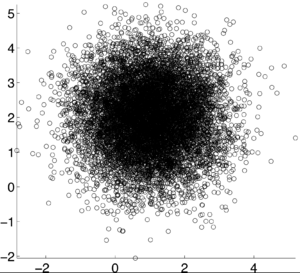
[[Image:correlation_coefficient_graph_pxy0.png|300px]] | [[Image:correlation_coefficient_graph_pxy0.png|300px]] | ||
| − | <math>\rho X,Y) = 0</math> [ | + | <math>\rho X,Y) = 0</math> [1] |
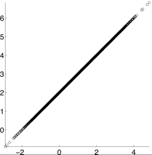
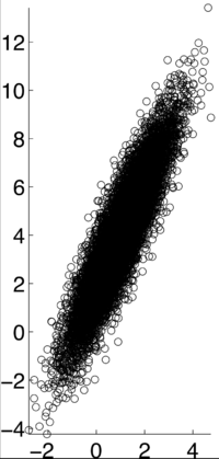
[[Image:correlation_coefficient_graph_pxy10.png|300px]] | [[Image:correlation_coefficient_graph_pxy10.png|300px]] | ||
| − | <math>\rho X,Y) = 1</math> [ | + | <math>\rho X,Y) = 1</math> [1] |
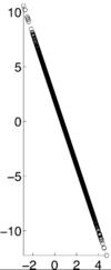
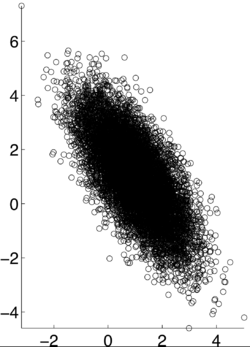
[[Image:correlation_coefficient_graph_pxy-10.png|100px]] | [[Image:correlation_coefficient_graph_pxy-10.png|100px]] | ||
| − | <math>\rho X,Y) = -1</math> [ | + | <math>\rho X,Y) = -1</math> [1] |
[[Image:correlation_coefficient_graph_pxy0_2.png|100px]] | [[Image:correlation_coefficient_graph_pxy0_2.png|100px]] | ||
| − | <math>\rho X,Y) = .2</math> [ | + | <math>\rho X,Y) = .2</math> [1] |
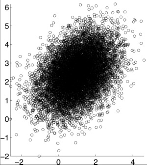
[[Image:correlation_coefficient_graph_pxy4.png|300px]] | [[Image:correlation_coefficient_graph_pxy4.png|300px]] | ||
| − | <math>\rho X,Y) = .4</math> [ | + | <math>\rho X,Y) = .4</math> [1] |
[[Image:correlation_coefficient_graph_pxy-7.png|250px]] | [[Image:correlation_coefficient_graph_pxy-7.png|250px]] | ||
| − | <math>\rho X,Y) = -.7</math> [ | + | <math>\rho X,Y) = -.7</math> [1] |
[[Image:correlation_coefficient_graph_pxy9.png|200px]] | [[Image:correlation_coefficient_graph_pxy9.png|200px]] | ||
| − | <math>\rho X,Y) = .9</math> [ | + | <math>\rho X,Y) = .9</math> [1] |
==Autocorrelation and Autocovariance== | ==Autocorrelation and Autocovariance== | ||
Correlation and covariance are comparing two random events. Autocorrelation and autocovariance are comparing the data points of one random event. | Correlation and covariance are comparing two random events. Autocorrelation and autocovariance are comparing the data points of one random event. | ||
| − | Autocovariance is defined as: <math> C_{s}(n1, n2) = E(X_{n1}X_{n2}) | + | Autocovariance is defined as: <math> C_{s}(n1, n2) = E(X_{n1}X_{n2}) </math> [2] |
| − | Autocorrelation is defined as: <math>R_{s}(n1, n2) = E((X_{n1}-E[X_{n1}])(X_{n2}-E[X_{n2}])) | + | Autocorrelation is defined as: <math>R_{s}(n1, n2) = E((X_{n1}-E[X_{n1}])(X_{n2}-E[X_{n2}])) </math>[2] |
---- | ---- | ||
Revision as of 19:12, 30 April 2013
Correlation vs Covariance
Student project for ECE302
by Blue
Contents
Correlation and Covariance
Correlation and covariance are very similarly related. Correlation is used to identify the relationship of two random variables, X and Y. In order to determine the dependence of the two events, the correlation coefficient,$ \rho $, is calculated as:
$ \rho (X,Y) = \frac{cov(X,Y)}{ \sqrt{var(X)var(Y)} } $
Covariance is defined as: $ C_{s}(n1, n2) = E(X-E[X])(Y-E[Y])) $ [1]
Correlation is then defined as: $ R_{s}(n1, n2) = E(XY) $ [2]
If X and Y are independent of each other, that means they are uncorrelated with each other, or cov(X,Y) = 0. However, if X and Y are uncorrelated, that does not mean they are independent of each other. 1, -1, and 0 are the three extreme points $ p\rho X,Y) $ can represent. 1 represents that X and Y are linearly dependent of each other. In other words, Y-E[Y] is a positive multiple of X-E[X]. -1 represents that X and Y are inversely dependent of each other. In other words, Y-E[Y] is a negative multiple of X-E[X]. [1]
Examples
Autocorrelation and Autocovariance
Correlation and covariance are comparing two random events. Autocorrelation and autocovariance are comparing the data points of one random event.
Autocovariance is defined as: $ C_{s}(n1, n2) = E(X_{n1}X_{n2}) $ [2]
Autocorrelation is defined as: $ R_{s}(n1, n2) = E((X_{n1}-E[X_{n1}])(X_{n2}-E[X_{n2}])) $[2]
References
[1]: Ilya Pollak. General Random Variables. 2012. Retrieved from https://engineering.purdue.edu/~ipollak/ece302/SPRING12/notes/19_GeneralRVs-4_Multiple_RVs.pdf
[2]: Ilya Pollak. Random Signals. 2004. Retrieved from https://engineering.purdue.edu/~ipollak/ee438/FALL04/notes/Section2.1.pdf

