| Line 1: | Line 1: | ||
| − | An impulse response, often denoted by h(t), is also called a transfer function or frequency response in frequency domain. It’s the output of In a LTI system when presented with a impulse signal input δ(t). In a LTI systems, impulse response is also equivalent to green’s function used in physics. | + | 1.An impulse response, often denoted by h(t), is also called a transfer function or frequency response in frequency domain. It’s the output of In a LTI system when presented with a impulse signal input δ(t). In a LTI systems, impulse response is also equivalent to green’s function used in physics. |
| + | |||
General theory of nth order ODE: | General theory of nth order ODE: | ||
An nth order linear differential equation is an equation of the form | An nth order linear differential equation is an equation of the form | ||
| + | |||
[[Image:Equation1.png]] | [[Image:Equation1.png]] | ||
| Line 15: | Line 17: | ||
A theorem states, if the functions p1, p2 …..,pn, and G are continuous on the open interval I, then there exists exactly one solution y = φ(t) of the differential equation (2) that also satisfies the initial conditions (3). | A theorem states, if the functions p1, p2 …..,pn, and G are continuous on the open interval I, then there exists exactly one solution y = φ(t) of the differential equation (2) that also satisfies the initial conditions (3). | ||
| + | |||
Source: Elementary differential eqution with boundary value problems by William E boyce. Ricahrd DeDrima | Source: Elementary differential eqution with boundary value problems by William E boyce. Ricahrd DeDrima | ||
| + | |||
| + | |||
| + | |||
| + | |||
| + | |||
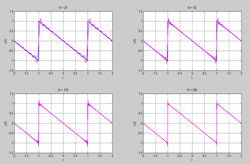
| + | 2. Illustration of Gibbs phenomenon: | ||
[[Image:bonus2matlab.png]] | [[Image:bonus2matlab.png]] | ||
| + | The overshoot increases as the number of terms increases, but approachs a finite limit. | ||
| + | |||
| + | Code: | ||
| + | t=linspace(-2,2,2000); | ||
| + | y=[sawtooth(-((t+1)*pi))]; | ||
| + | N=[25,50,150,500]; | ||
| + | for i=1:4; | ||
| + | an=[]; | ||
| + | for m=1:N(i) | ||
| + | an=[an,4*cos(m*pi/2)/(m*pi)]; | ||
| + | end; | ||
| + | fn=0; | ||
| + | for m=1:N(i) | ||
| + | fn=fn+an(m)*sin(m*pi/2*t); | ||
| + | end; | ||
| + | subplot(2,2,i) | ||
| + | plot(t,y,'LineWidth',2); | ||
| + | hold on; | ||
| + | plot(t,fn,'m','LineWidth',2); | ||
| + | hold off; | ||
| + | axis([-2 2 -1.5 1.5]); | ||
| + | grid; | ||
| + | xlabel('t'), ylabel('y(t)');title(['N = ',int2str(N(i))]); | ||
| + | end; | ||
| + | |||
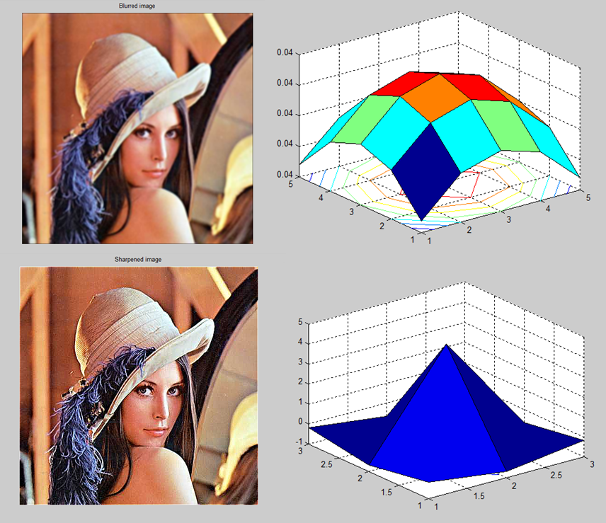
| + | 3. Spatial image filtering operations: | ||
| + | |||
[[Image:bonus2image.png]] | [[Image:bonus2image.png]] | ||
| + | |||
| + | Code: | ||
| + | clc | ||
| + | clear all | ||
| + | img = imread('Lena.jpg') | ||
| + | f = fspecial('gaussian',[5 5],100); | ||
| + | imgGaussian = imfilter(img,f); | ||
| + | figure; imshow(img); title('Original'); | ||
| + | figure; imshow(imgGaussian); title('Blurred image') | ||
| + | figure; surfc(f) | ||
| + | s = fspecial('unsharp'); | ||
| + | imgSharp = imfilter(img, s); | ||
| + | figure; imshow(imgSharp); title('Sharpened image') | ||
| + | figure; surfc(s) | ||
Revision as of 22:34, 10 March 2013
1.An impulse response, often denoted by h(t), is also called a transfer function or frequency response in frequency domain. It’s the output of In a LTI system when presented with a impulse signal input δ(t). In a LTI systems, impulse response is also equivalent to green’s function used in physics.
General theory of nth order ODE:
An nth order linear differential equation is an equation of the form
Divide by Po(t) to get the following form
Has n initial conditions
A theorem states, if the functions p1, p2 …..,pn, and G are continuous on the open interval I, then there exists exactly one solution y = φ(t) of the differential equation (2) that also satisfies the initial conditions (3).
Source: Elementary differential eqution with boundary value problems by William E boyce. Ricahrd DeDrima
2. Illustration of Gibbs phenomenon:
The overshoot increases as the number of terms increases, but approachs a finite limit.
Code: t=linspace(-2,2,2000); y=[sawtooth(-((t+1)*pi))]; N=[25,50,150,500]; for i=1:4; an=[]; for m=1:N(i) an=[an,4*cos(m*pi/2)/(m*pi)]; end; fn=0; for m=1:N(i) fn=fn+an(m)*sin(m*pi/2*t); end; subplot(2,2,i) plot(t,y,'LineWidth',2); hold on; plot(t,fn,'m','LineWidth',2); hold off; axis([-2 2 -1.5 1.5]); grid; xlabel('t'), ylabel('y(t)');title(['N = ',int2str(N(i))]); end;
3. Spatial image filtering operations:
Code: clc clear all img = imread('Lena.jpg') f = fspecial('gaussian',[5 5],100); imgGaussian = imfilter(img,f); figure; imshow(img); title('Original'); figure; imshow(imgGaussian); title('Blurred image') figure; surfc(f) s = fspecial('unsharp'); imgSharp = imfilter(img, s); figure; imshow(imgSharp); title('Sharpened image') figure; surfc(s)


