| (5 intermediate revisions by the same user not shown) | |||
| Line 20: | Line 20: | ||
==Problem 1== | ==Problem 1== | ||
| − | + | 1. Calcualte an expression for <math>\lambda_n^c</math>, the X-ray energy corrected for the dark current | |
<center> | <center> | ||
| Line 26: | Line 26: | ||
</center> | </center> | ||
| − | + | 2. Calculate an expression for <math>G_n</math>, the X-ray attenuation due to the object's presence | |
<center> | <center> | ||
| Line 32: | Line 32: | ||
</center> | </center> | ||
| − | + | 3. Calculate an expression for <math>\hat{P}_n</math>, an estimate of the integral intensity in terms of <math>\lambda_n</math>, <math>\lambda_n^b</math>, and <math>\lambda_n^d</math> | |
| Line 41: | Line 41: | ||
</center> | </center> | ||
| − | + | 4. For this part, assume that the object is of constant density with <math>\mu(x,y) = \mu_0</math>. Then sketch a plot of <math>\hat{P}_n</math> versus the object thickness, <math>T_n</math>, in mm, for the <math>n^{th}</math> detector. Label key features of the curve such as its slope and intersection. | |
| + | |||
| + | [[Image:cs52016.jpg]] | ||
==Problem 2== | ==Problem 2== | ||
| − | + | 1. Specify the size of <math>YY^t</math> and <math>Y^tY</math>. Which matrix is smaller | |
<center> | <center> | ||
| Line 55: | Line 57: | ||
</center> | </center> | ||
| − | + | 2. Prove that both <math>YY^t</math> and <math>Y^tY</math> are both symmetric and positive semi-definite matrices. | |
<center> | <center> | ||
| Line 71: | Line 73: | ||
</center> | </center> | ||
| − | + | 3. Derive expressions for <math>V</math> and <math>\Sigma</math> in terms of <math>T</math>, and <math>D</math>. | |
<center> | <center> | ||
| Line 77: | Line 79: | ||
</center> | </center> | ||
| − | + | 4. Derive an expression for <math>U</math> in terms of <math>Y</math>, <math>T</math>, <math>D</math>. | |
<center> | <center> | ||
| Line 85: | Line 87: | ||
</center> | </center> | ||
| − | + | 5. Derive expressions for E in terms of Y, T, and D. | |
<center> | <center> | ||
<math>YY^t = U\Sigma V^t(U\Sigma V^t)^t= U\Sigma^2 U^t = E\Gamma E^t</math> | <math>YY^t = U\Sigma V^t(U\Sigma V^t)^t= U\Sigma^2 U^t = E\Gamma E^t</math> | ||
| Line 94: | Line 96: | ||
</center> | </center> | ||
| − | + | 6. If the columns of Y are images from a training database, then what name do we give to the columns of U? | |
<center> | <center> | ||
| − | They are called '''eigenimages''' | + | They are called '''eigenimages'''. |
</center> | </center> | ||
Latest revision as of 02:07, 26 April 2020
Communication, Networking, Signal and Image Processing (CS)
Question 5: Image Processing
August 2016 (Published in Jul 2019)
Problem 1
1. Calcualte an expression for $ \lambda_n^c $, the X-ray energy corrected for the dark current
$ \lambda_n^c=\lambda_n^b-\lambda_n^d $
2. Calculate an expression for $ G_n $, the X-ray attenuation due to the object's presence
$ G_n = \frac{d\lambda_n^c}{dx}=-\mu (x,y_0+n * \Delta d)\lambda_n^c $
3. Calculate an expression for $ \hat{P}_n $, an estimate of the integral intensity in terms of $ \lambda_n $, $ \lambda_n^b $, and $ \lambda_n^d $
$ \lambda_n = (\lambda_n^b-\lambda_n^d) e^{-\int_{0}^{x}\mu(t)dt}d)\lambda_n^c $
$ \hat{P}_n = \int_{0}^{x}\mu(t)dt= -log(\frac{\lambda_n}{\lambda_n^b-\lambda_n^d}) $
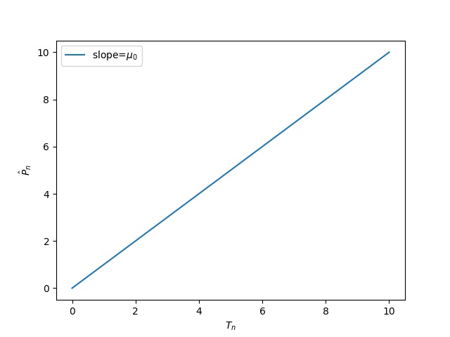
4. For this part, assume that the object is of constant density with $ \mu(x,y) = \mu_0 $. Then sketch a plot of $ \hat{P}_n $ versus the object thickness, $ T_n $, in mm, for the $ n^{th} $ detector. Label key features of the curve such as its slope and intersection.
Problem 2
1. Specify the size of $ YY^t $ and $ Y^tY $. Which matrix is smaller
Y is of size $ p \times N $, so the size of $ YY^t $ is $ p \times p $
Y is of size $ p \times N $, so the size of $ Y^tY $ is $ N \times N $
Obviously, the size of $ Y^tY $ is much smaller, since N << p.
2. Prove that both $ YY^t $ and $ Y^tY $ are both symmetric and positive semi-definite matrices.
To prove it is symmetric:
$ (YY^t)^t = YY^t $
To prove it is positive semi-definite:
Let x be an arbitrary vector
$ x^tYY^tx = (Y^tx)^T(Y^tx) \geq 0 $ so the matrix of $ YY^t $ is positive semi-definite.
The proving procedures for $ Y^tY $ are the same
3. Derive expressions for $ V $ and $ \Sigma $ in terms of $ T $, and $ D $.
$ Y^tY = (U \Sigma V^t)^T U \Sigma V^t = V\Sigma^2 V^t = TDT^t $ therefore $ V =T $ and $ \Sigma = D^{\frac{1}{2}} $
4. Derive an expression for $ U $ in terms of $ Y $, $ T $, $ D $.
$ Y = U\Sigma V^t= UD^{\frac{1}{2}}T^t $
$ \therefore U = Y(D^{\frac{1}{2}}T^t)^{-1} $
5. Derive expressions for E in terms of Y, T, and D.
$ YY^t = U\Sigma V^t(U\Sigma V^t)^t= U\Sigma^2 U^t = E\Gamma E^t $
therefore
$ E = U = Y(D^{\frac{1}{2}}T^t)^{-1} $
6. If the columns of Y are images from a training database, then what name do we give to the columns of U?
They are called eigenimages.


