| (3 intermediate revisions by the same user not shown) | |||
| Line 1: | Line 1: | ||
==Introduction== | ==Introduction== | ||
| − | In sound systems it is often desirable to have a flat frequency response along the range of human hearing (20Hz - 20kHz). While this goal can be easily achieved for a single loudspeaker system, it is challenging to achieve a perfectly flat response in | + | In sound systems it is often desirable to have a flat frequency response along the range of human hearing (20Hz - 20kHz). While this goal can be easily achieved for a single loudspeaker system, it is challenging to achieve a perfectly flat response in multi-speaker systems. In the large venues where multi-speaker sound reinforcement systems are necessary it is possible for the frequency response in one location be vastly different from the response in another. Summation effects from the multiple sources can lead to significant spatial variance in the frequency response. If two audio sources are at a similar level and significantly out of phase (150 - 210 degrees)they can cancel resulting in audible "dead zones". |
==Application of class material== | ==Application of class material== | ||
| − | + | Through careful consideration to the location and aiming angle of the speakers it is possible to design a system that avoids these "dead zones". However even in the most carefully designed systems it is impossible to achieve perfect uniformity across the listening space. It is therefore desirable to be able to measure the frequency response of the system at multiple locations in order to fine tune the system. Matlab can be used to show a plot of the frequency response at different locations. The script below allows the user to easily define the number of sampling locations desired, and use a microphone to record samples of the sound at each point. A FFT is then used to plot and graph the power spectral density vs frequency at that location. By playing pink noise (sound that has equal energy per octave) through the system it is possible to find locations where the audio quality has been negatively impacted by summation effects. | |
==Code== | ==Code== | ||
| − | [[File:438code. | + | [[File:438code.PNG|thumbnail]] |
| + | |||
| + | ==References== | ||
| + | D.G. Meyer https://engineering.purdue.edu/ece40020/LectureNotes/Ch_02_LS.pdf | ||
Latest revision as of 23:06, 23 April 2017
Introduction
In sound systems it is often desirable to have a flat frequency response along the range of human hearing (20Hz - 20kHz). While this goal can be easily achieved for a single loudspeaker system, it is challenging to achieve a perfectly flat response in multi-speaker systems. In the large venues where multi-speaker sound reinforcement systems are necessary it is possible for the frequency response in one location be vastly different from the response in another. Summation effects from the multiple sources can lead to significant spatial variance in the frequency response. If two audio sources are at a similar level and significantly out of phase (150 - 210 degrees)they can cancel resulting in audible "dead zones".
Application of class material
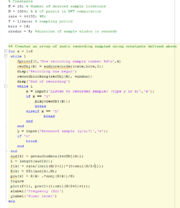
Through careful consideration to the location and aiming angle of the speakers it is possible to design a system that avoids these "dead zones". However even in the most carefully designed systems it is impossible to achieve perfect uniformity across the listening space. It is therefore desirable to be able to measure the frequency response of the system at multiple locations in order to fine tune the system. Matlab can be used to show a plot of the frequency response at different locations. The script below allows the user to easily define the number of sampling locations desired, and use a microphone to record samples of the sound at each point. A FFT is then used to plot and graph the power spectral density vs frequency at that location. By playing pink noise (sound that has equal energy per octave) through the system it is possible to find locations where the audio quality has been negatively impacted by summation effects.
Code
References
D.G. Meyer https://engineering.purdue.edu/ece40020/LectureNotes/Ch_02_LS.pdf


