| (27 intermediate revisions by 3 users not shown) | |||
| Line 1: | Line 1: | ||
== Introduction == | == Introduction == | ||
| + | The allocation of scarce resources is a universal issue, and the goal is usually to do so in an optimal way. The ability to transport goods at an optimal cost is of particular interest to both businesses and individuals. Linear programming is a method of allocating resources in an optimal way; and it is one of the most widely used tools for decision making in manufacturing industries. | ||
| − | + | In the term '''linear programming''', programming refers to mathematical programming. In this context, it refers to a process which allocates resources in the best possible (optimal) way; to minimize costs or to maximize profits. In linear programming, the resources to be allocated are known as '''decision variables'''. The criterion for choosing the best values of the decision variables is known as the '''objective function'''. Restrictions on the availability of resources form what is known as a '''constraint set'''. | |
| − | + | The word linear indicates that the criteria for choosing optimal values of the decision variables can be described by a linear function of these variables; i.e., a function involving only the first powers of the decision variables, and no products of the variables. Thus the entire problem can be expressed in terms of straight lines, planes, or similar geometric figures. In addition to the linear requirements, there is a restriction of non-negativity; i.e., it is impossible to have negative resources. | |
| − | + | One of the most important applications of linear programming has been in the physical distribution of goods, commonly referred to as '''transportation problems'''. Essentially, the purpose is to minimize the cost of shipping goods from one location to another in such a way that the needs of each destination is met and each shipping location operates within its capacity. | |
| − | |||
| − | Conclusion | + | == Formulation & Mathematical Model of a Transportation Problem == |
| + | |||
| + | The best way to go about understanding the mathematics behind the transportation problem is to think of a real-life example. Let’s say a clothing company has ''m'' warehouses, where the goods are produced. The company also has "n" outlet stores, where the goods will be sold. We know there exist m warehouses and n outlet stores, but we need to explicitly label each one. We label the warehouses as: | ||
| + | |||
| + | <math>i=1,2,...,m</math> | ||
| + | |||
| + | And we label the outlet stores as: | ||
| + | |||
| + | <math>j = 1, 2, ... , n</math> | ||
| + | |||
| + | Now this is where Supply and Demand come into play. The warehouses have a level of supply and the outlet stores have a level of demand that need to be met. We can define the supply of each warehouse as <math>a_i</math> and the demand of each outlet store as <math>b_j</math>. Now, the question is what are we trying to calculate? In simplest terms, the transportation problem is an optimization problem. In our case, we want to get good from the warehouses to the outlet stores at minimum cost. Knowing this, and assuming that the cost of shipping is linear, we can define shipping cost from the i<sup>th</sup> warehouse to the j<sup>th</sup> outlet store as <math>c_{ij}</math>. The last thing that needs to be defined is the number of units transported from the i<sup>th</sup> warehouse to the j<sup>th</sup>, which we can call <math>x_{ij}</math>. Now, we have all of the terms we'll need to begin solving the problem. | ||
| + | |||
| + | A quick recap of what is written above: | ||
| + | * m and n are defined as the number of sources and the number of destinations, respectively (warehouses and outlet stores in our example) | ||
| + | * The goods produced at the i<sup>th</sup> source is defined as <math>a_i</math> | ||
| + | * The demand at the j<sup>th</sup> destination is defined as <math>b_j</math> | ||
| + | * <math>c_{ij}</math> is defined as the shipping cost when being shipped from i to j | ||
| + | * <math>x_{ij}</math> is defined as the number of units being shipped from source i to destination j | ||
| + | Note: <math>x_{ij}\geq 0</math>; you can’t have a negative number of units. | ||
| + | |||
| + | Now we need to ask, what do we do with all of these terms? The initial setup of the problem is actually fairly easy. Say, for example, we want to transport 2 shipments of 5 shirts from our warehouses to 2 outlet stores, where one shipment goes to one outlet store, and it costs $1 to ship each shirt. We know that it costs a total of $5 per shipment (cost of shipment x number of units) and there are 2 shipments, so summing them, it’s $10 total. Fairly simple. Expressed mathematically, we can use sums to give ourselves a formula: | ||
| + | |||
| + | <math>\sum_{i=1}^m \sum_{j=1}^n c_{ij}x_{ij}</math> | ||
| + | |||
| + | The goal is to minimize this equation. However, there are some constraints that exist. Let’s say the warehouse is again shipping 2 shipments of 5 shirts. However, the warehouse only has 8 shirts in-house. Can the warehouse ship its required 10 shirts? The obvious answer is no, since they only have 8 shirts available. So the first constraint is that units being shipped cannot exceed the supply available. Mathematically, this can be expressed as: | ||
| + | |||
| + | <math>\sum_{j=1}^n x_{ij}\leq a_i; i=1,2,...,m</math> | ||
| + | |||
| + | There is a similar constraint for demand demand. However, the problem with the demand is not overselling products you don’t have. Instead, the issue is not having enough supply to meet the demand. This can be expressed as: | ||
| + | |||
| + | <math>\sum_{i=1}^m x_{ij}\geq b_j; j=1,2,...,n</math> | ||
| + | |||
| + | To summarize, we want to minimize | ||
| + | |||
| + | <math>\sum_{i=1}^m \sum_{j=1}^n c_{ij}x_{ij}</math> | ||
| + | |||
| + | With the constraints: | ||
| + | |||
| + | <math>\sum_{j=1}^n x_{ij}\leq a_i; i=1,2,...,m</math> | ||
| + | |||
| + | <math>\sum_{i=1}^m x_{ij}\geq b_j; j=1,2,...,n</math> | ||
| + | |||
| + | <math>x_{ij}\geq 0, \forall i \in \{1,2,...,m\}, j \in \{1,2,...,n\}</math> | ||
| + | |||
| + | A conclusion we can draw from the information above is that the only way that the problem makes sense is if the supply exceeds or equals the demand. Otherwise the constraints would not be met, namely supply would not meet demand. Knowing that supply must equal or exceed demand, it’s safe to assume that any surplus can be ignored. Thus we can state the following: | ||
| + | |||
| + | <math>\sum_{j=1}^n a_i = \sum_{i=1}^m b_j</math> | ||
| + | |||
| + | Which says that total supply and total demand should be equal. | ||
| + | |||
| + | '''Other ways to think about the transportation problem:''' | ||
| + | |||
| + | While the above illustrates the main mathematics behind the transportation problem, there are other ways to interpret the problem. One way we can do this is looking at the problem from a graphical standpoint. | ||
| + | |||
| + | Let’s look at waste and recycling transport. In a city, there are 4 districts and 2 landfills, where there is a maximum amount of trash that can be put in each landfill, also know as the demand. Each district has a supply of trash that needs to be moved to the landfills. | ||
| + | |||
| + | [[File:Rsz nodepic.png]] | ||
| + | |||
| + | Each circle on the left, called a node, represents a district, specifically called a '''source node''' and each node on the left, is referred to as a '''destination node''', and represents the landfills. The numbers on either side of the nodes are the '''capacity''' of each node while the numbers on the arrows are the '''per-unit cost''' of shipping from one source node to a destination node. As you can see, the numbers in red exemplify the cheapest shipping cost, while it does not necessarily represent the ideal destination, based on capacity. | ||
| + | |||
| + | We can use this graphical representation to then create a table which is known as a '''transportation matrix''' or '''transportation model'''. Let's label the first source node 1, the second one 2 and so on. We do the same with the destination nodes. A table can be made that looks like the following: | ||
| + | |||
| + | [[File:Rsz transportationmodeltable1.PNG]] | ||
| + | |||
| + | It's easy to see what each number represents, as everything is explicitly labeled in the table. For example, we know that to get the garbage from city district 1 to landfill 2, it costs 5 units, which lines up with the graphical representation from earlier. Notice how the last column and row are labeled "supply" and "demand". These aren't always what they need to be labeled. For example, they could be labeled "output" and "requirement". | ||
| + | |||
| + | Now the question is, what do we do with this table? How does it help us solve our problem? This is where the minimization comes in. Let <math>x_{ij}</math> be the number of shipments from district ''i'' to landfill ''j''. We can set up the minimization like so: | ||
| + | |||
| + | ''minimize'' → 2<math>x_{11}</math> + 5<math>x_{12}</math> + 3<math>x_{21}</math> + ... + 1<math>x_{42}</math> | ||
| + | |||
| + | ''with the constraints'': | ||
| + | |||
| + | <math>x_{11}</math> + <math>x_{12}</math> = 500 | ||
| + | |||
| + | <math>x_{21}</math> + <math>x_{22}</math> = 750 | ||
| + | |||
| + | <math>x_{31}</math> + <math>x_{32}</math> = 1500 | ||
| + | |||
| + | <math>x_{41}</math> + <math>x_{42}</math> = 750 | ||
| + | |||
| + | <math>x_{11}</math> + <math>x_{21}</math> + <math>x_{31}</math> + <math>x_{41}</math> = 2000 | ||
| + | |||
| + | <math>x_{12}</math> + <math>x_{22}</math> + <math>x_{23}</math> + <math>x_{24}</math> = 1000 | ||
| + | |||
| + | The setup of these equations is just intuition and making sure you get the right numbers in the right spots. | ||
| + | |||
| + | |||
| + | == How to Solve the Transportation Problem with an Example == | ||
| + | |||
| + | Before beginning the example, here is a quick preview of the method we will be using, called the '''Vogel Approximation Method''', or '''VAM'''. The VAM method uses tables like the one in the previous section and is solved through 5 steps: | ||
| + | |||
| + | 1) Find the difference between the lowest two cells in the rows and columns | ||
| + | |||
| + | 2) Figure out which row or column has the largest difference (Note: ties can happen in a situation like this. In this case, determine a tie-breaker through any mean, it's not important how the winner is chosen) | ||
| + | |||
| + | 3) Assign, as much as possible, this column/row with the largest difference to the lowest-cost cell | ||
| + | |||
| + | 4) If all demand or requirement is met, then you're done. However, if not, continue with the next step. | ||
| + | |||
| + | 5) Again, calculate the differences between the two lowest row or column remaining in all rows and columns. (Note: if any row or column equals 0, it should not be used in calculating the differences). Go back to step 2 and repeat until all the demand/requirements are met. | ||
| + | |||
| + | |||
| + | The easiest way to understand this methodology is to see it in motion, so now, let us put solving the transportation problem into practice with a simple example. | ||
| + | |||
| + | Jack, Jill, and John all have fruit stands that stock apples, oranges, and bananas. They are supplied by three farmers (Farmers A, B, C). Farmer A grows apples, Farmer B grows bananas, and Farmer C grows oranges. The following table gives the cost of transporting one pound of fruit to a fruit stand: | ||
| + | |||
| + | [[File:Vam example table.PNG]] | ||
| + | |||
| + | Jack needs at least 30 lbs of fruit, Jill needs at least 30 lbs of fruit, and Joe needs at least 20 lbs of fruit. Farmer A can only supply 30 lbs of apples, Farmer B can only supply 30 lbs of bananas, and Farmer C can only supply 20 lbs of oranges. How many pounds of each fruit should each person get in order to minimize the cost of transportation? | ||
| + | |||
| + | For a small problem such as this, the first step to solving is setting up a table with the constraints. We will include the per-unit costs as well (lower right corners), and a “row difference” and “column difference”. The row difference is the difference between the second-lowest and lowest transportation cost for that item. For example, the lowest cost in the apples row is $3 (shipping to Jack), and the second lowest is $5 (shipping to Jill), so the value in the row difference box for apples is $5-$3 = $2. Similarly for the column difference, for Jack, the column difference is $4-$3 = $1. | ||
| + | |||
| + | [[File:Vam step 1.PNG]] | ||
| + | |||
| + | Now that the table is set up, we can begin solving. First, we find the highest value from the row and column differences. For this example, the highest value is $3 in Jill’s column (Note; if there were multiple of the highest value, choosing the starting one is arbitrary). Using that column, we go to the row with the lowest cost, and assign as much of that item to her as we can. So for Jill, we assign her 20 pounds of oranges, and that is the most we can ship of oranges. This leaves no oranges available for anyone else (we can assign Jack and John zero oranges), and Jill now only needs 10 more pounds of fruit. We indicate these changes on the table in red: | ||
| + | |||
| + | [[File:Vam step 2.PNG]] | ||
| + | |||
| + | We can now consider the oranges row ‘done’. The next step is to reassign row and column difference values ignoring the costs in the oranges row. As no changes were made to the apples or bananas rows, their row difference values remain unchanged. However, the column differences are different. The differences become $6-$3 = $3 for Jack, $6-$5 = $1 for Jill, and $9-$7 = $2 for John. The changed values are marked in red in the table: | ||
| + | |||
| + | [[File:Vam step 3.PNG]] | ||
| + | |||
| + | We repeat the fruit assignment step, giving as much fruit as constraints allow to the smallest cost in the row/column of the highest difference value. In this case, Jack gets 30 lbs of apples, which is all the fruit he needs and all the apples available. We mark the necessary changes to the table in red: | ||
| + | |||
| + | [[File:Vam step 4.PNG]] | ||
| + | |||
| + | After this assignment, there are only two boxes (Jill-bananas and John-bananas) without assigned values. This allows us to do our final assignment without calculating row and column differences. We simply assign as much as we can to the cheapest option, then the remainder to the other. Of the remaining 30 lbs of bananas, Jill gets 10 lbs, bringing her needed fruit to zero and leaving 20 lbs of bananas for John, bringing his needed fruit to zero. The final assignment is as follows: | ||
| + | |||
| + | [[File:Vam final assignment.PNG]] | ||
| + | |||
| + | We find the total cost by taking the pounds of each fruit each person gets times the per unit cost of transporting that fruit to that person. Total cost = ($3*30 + $5*0 + $7*0 ) + ($6*0 + $6*10 + $9*20) + ($4*0 + $2*20 + $8*0) = $370. | ||
| + | The Vogel Approximation Method often produces the optimal solution. Examining our solution for this example, we can see that changing the amounts of fruits anyone gets would lead to a higher cost, and thus our solution is optimal. | ||
| + | |||
| + | |||
| + | == Conclusion == | ||
| + | |||
| + | The transportation problem is a very special case when it comes to linear programming. As seen above, these problems can be time-consuming and very easy to make computational areas in, so in real-life applications, they would most likely be done by a computer. While initially the transportation problem was developed to solve problems in transporting goods from one the source to the destination, the transportation method can be used to solve other problems, such as what is referred to as an '''assignment problem'''. The assignment problem deals with the same concept but instead of transporting goods, it is used to assign people to jobs, machines, etc. Another application of the transportation problem is it can be used for things like scheduling as well. The only constraint in non-transporting problems is you have to be able to set up it up as a transportation matrix, or else there would be no way to solving the problem. | ||
| + | |||
| + | |||
| + | == References == | ||
| + | Dwyer, Paul S. The Direct Solution of the Transportation Problem with Reduced Matrices 13.1 (1966): 77-96. Institute for Operations Research and the Management Sciences. Web. Apr. 2016. | ||
| + | |||
| + | Havelick, Jaroslav, and Ludmila Domeova. "The Transportation Problem." Distance Learning Module for Management Science. N.p., n.d. Web. 21 Apr. 2016. | ||
| + | |||
| + | Reeb, James E., and Scott A. Leavengood. Transportation Problem: A Special Case for Linear Programming Problems. Corvallis, Or.: Oregon State U Extension Service, 2002. Web. Apr. 2016. | ||
| + | |||
| + | "Transportation Problem in Excel." Easy Excel Tutorial. Excel Easy, 2010. Web. 24 Apr. 2016. | ||
| + | |||
| + | Trick, Michael A. "Transportation Problem." Transportation Problem. N.p., 24 Aug. 1998. Web. 24 Apr. 2016. | ||
| + | |||
| + | |||
| + | [[Category:MA279Spring2016Walther]] | ||
Latest revision as of 21:35, 24 April 2016
Contents
Introduction
The allocation of scarce resources is a universal issue, and the goal is usually to do so in an optimal way. The ability to transport goods at an optimal cost is of particular interest to both businesses and individuals. Linear programming is a method of allocating resources in an optimal way; and it is one of the most widely used tools for decision making in manufacturing industries.
In the term linear programming, programming refers to mathematical programming. In this context, it refers to a process which allocates resources in the best possible (optimal) way; to minimize costs or to maximize profits. In linear programming, the resources to be allocated are known as decision variables. The criterion for choosing the best values of the decision variables is known as the objective function. Restrictions on the availability of resources form what is known as a constraint set.
The word linear indicates that the criteria for choosing optimal values of the decision variables can be described by a linear function of these variables; i.e., a function involving only the first powers of the decision variables, and no products of the variables. Thus the entire problem can be expressed in terms of straight lines, planes, or similar geometric figures. In addition to the linear requirements, there is a restriction of non-negativity; i.e., it is impossible to have negative resources.
One of the most important applications of linear programming has been in the physical distribution of goods, commonly referred to as transportation problems. Essentially, the purpose is to minimize the cost of shipping goods from one location to another in such a way that the needs of each destination is met and each shipping location operates within its capacity.
Formulation & Mathematical Model of a Transportation Problem
The best way to go about understanding the mathematics behind the transportation problem is to think of a real-life example. Let’s say a clothing company has m warehouses, where the goods are produced. The company also has "n" outlet stores, where the goods will be sold. We know there exist m warehouses and n outlet stores, but we need to explicitly label each one. We label the warehouses as:
$ i=1,2,...,m $
And we label the outlet stores as:
$ j = 1, 2, ... , n $
Now this is where Supply and Demand come into play. The warehouses have a level of supply and the outlet stores have a level of demand that need to be met. We can define the supply of each warehouse as $ a_i $ and the demand of each outlet store as $ b_j $. Now, the question is what are we trying to calculate? In simplest terms, the transportation problem is an optimization problem. In our case, we want to get good from the warehouses to the outlet stores at minimum cost. Knowing this, and assuming that the cost of shipping is linear, we can define shipping cost from the ith warehouse to the jth outlet store as $ c_{ij} $. The last thing that needs to be defined is the number of units transported from the ith warehouse to the jth, which we can call $ x_{ij} $. Now, we have all of the terms we'll need to begin solving the problem.
A quick recap of what is written above:
- m and n are defined as the number of sources and the number of destinations, respectively (warehouses and outlet stores in our example)
- The goods produced at the ith source is defined as $ a_i $
- The demand at the jth destination is defined as $ b_j $
- $ c_{ij} $ is defined as the shipping cost when being shipped from i to j
- $ x_{ij} $ is defined as the number of units being shipped from source i to destination j
Note: $ x_{ij}\geq 0 $; you can’t have a negative number of units.
Now we need to ask, what do we do with all of these terms? The initial setup of the problem is actually fairly easy. Say, for example, we want to transport 2 shipments of 5 shirts from our warehouses to 2 outlet stores, where one shipment goes to one outlet store, and it costs $1 to ship each shirt. We know that it costs a total of $5 per shipment (cost of shipment x number of units) and there are 2 shipments, so summing them, it’s $10 total. Fairly simple. Expressed mathematically, we can use sums to give ourselves a formula:
$ \sum_{i=1}^m \sum_{j=1}^n c_{ij}x_{ij} $
The goal is to minimize this equation. However, there are some constraints that exist. Let’s say the warehouse is again shipping 2 shipments of 5 shirts. However, the warehouse only has 8 shirts in-house. Can the warehouse ship its required 10 shirts? The obvious answer is no, since they only have 8 shirts available. So the first constraint is that units being shipped cannot exceed the supply available. Mathematically, this can be expressed as:
$ \sum_{j=1}^n x_{ij}\leq a_i; i=1,2,...,m $
There is a similar constraint for demand demand. However, the problem with the demand is not overselling products you don’t have. Instead, the issue is not having enough supply to meet the demand. This can be expressed as:
$ \sum_{i=1}^m x_{ij}\geq b_j; j=1,2,...,n $
To summarize, we want to minimize
$ \sum_{i=1}^m \sum_{j=1}^n c_{ij}x_{ij} $
With the constraints:
$ \sum_{j=1}^n x_{ij}\leq a_i; i=1,2,...,m $
$ \sum_{i=1}^m x_{ij}\geq b_j; j=1,2,...,n $
$ x_{ij}\geq 0, \forall i \in \{1,2,...,m\}, j \in \{1,2,...,n\} $
A conclusion we can draw from the information above is that the only way that the problem makes sense is if the supply exceeds or equals the demand. Otherwise the constraints would not be met, namely supply would not meet demand. Knowing that supply must equal or exceed demand, it’s safe to assume that any surplus can be ignored. Thus we can state the following:
$ \sum_{j=1}^n a_i = \sum_{i=1}^m b_j $
Which says that total supply and total demand should be equal.
Other ways to think about the transportation problem:
While the above illustrates the main mathematics behind the transportation problem, there are other ways to interpret the problem. One way we can do this is looking at the problem from a graphical standpoint.
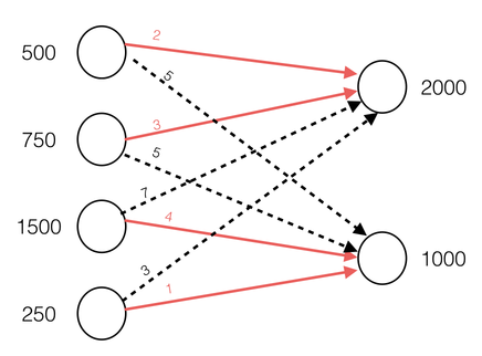
Let’s look at waste and recycling transport. In a city, there are 4 districts and 2 landfills, where there is a maximum amount of trash that can be put in each landfill, also know as the demand. Each district has a supply of trash that needs to be moved to the landfills.
Each circle on the left, called a node, represents a district, specifically called a source node and each node on the left, is referred to as a destination node, and represents the landfills. The numbers on either side of the nodes are the capacity of each node while the numbers on the arrows are the per-unit cost of shipping from one source node to a destination node. As you can see, the numbers in red exemplify the cheapest shipping cost, while it does not necessarily represent the ideal destination, based on capacity.
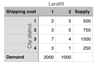
We can use this graphical representation to then create a table which is known as a transportation matrix or transportation model. Let's label the first source node 1, the second one 2 and so on. We do the same with the destination nodes. A table can be made that looks like the following:
It's easy to see what each number represents, as everything is explicitly labeled in the table. For example, we know that to get the garbage from city district 1 to landfill 2, it costs 5 units, which lines up with the graphical representation from earlier. Notice how the last column and row are labeled "supply" and "demand". These aren't always what they need to be labeled. For example, they could be labeled "output" and "requirement".
Now the question is, what do we do with this table? How does it help us solve our problem? This is where the minimization comes in. Let $ x_{ij} $ be the number of shipments from district i to landfill j. We can set up the minimization like so:
minimize → 2$ x_{11} $ + 5$ x_{12} $ + 3$ x_{21} $ + ... + 1$ x_{42} $
with the constraints:
$ x_{11} $ + $ x_{12} $ = 500
$ x_{21} $ + $ x_{22} $ = 750
$ x_{31} $ + $ x_{32} $ = 1500
$ x_{41} $ + $ x_{42} $ = 750
$ x_{11} $ + $ x_{21} $ + $ x_{31} $ + $ x_{41} $ = 2000
$ x_{12} $ + $ x_{22} $ + $ x_{23} $ + $ x_{24} $ = 1000
The setup of these equations is just intuition and making sure you get the right numbers in the right spots.
How to Solve the Transportation Problem with an Example
Before beginning the example, here is a quick preview of the method we will be using, called the Vogel Approximation Method, or VAM. The VAM method uses tables like the one in the previous section and is solved through 5 steps:
1) Find the difference between the lowest two cells in the rows and columns
2) Figure out which row or column has the largest difference (Note: ties can happen in a situation like this. In this case, determine a tie-breaker through any mean, it's not important how the winner is chosen)
3) Assign, as much as possible, this column/row with the largest difference to the lowest-cost cell
4) If all demand or requirement is met, then you're done. However, if not, continue with the next step.
5) Again, calculate the differences between the two lowest row or column remaining in all rows and columns. (Note: if any row or column equals 0, it should not be used in calculating the differences). Go back to step 2 and repeat until all the demand/requirements are met.
The easiest way to understand this methodology is to see it in motion, so now, let us put solving the transportation problem into practice with a simple example.
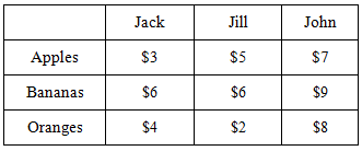
Jack, Jill, and John all have fruit stands that stock apples, oranges, and bananas. They are supplied by three farmers (Farmers A, B, C). Farmer A grows apples, Farmer B grows bananas, and Farmer C grows oranges. The following table gives the cost of transporting one pound of fruit to a fruit stand:
Jack needs at least 30 lbs of fruit, Jill needs at least 30 lbs of fruit, and Joe needs at least 20 lbs of fruit. Farmer A can only supply 30 lbs of apples, Farmer B can only supply 30 lbs of bananas, and Farmer C can only supply 20 lbs of oranges. How many pounds of each fruit should each person get in order to minimize the cost of transportation?
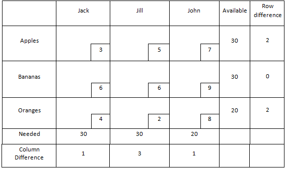
For a small problem such as this, the first step to solving is setting up a table with the constraints. We will include the per-unit costs as well (lower right corners), and a “row difference” and “column difference”. The row difference is the difference between the second-lowest and lowest transportation cost for that item. For example, the lowest cost in the apples row is $3 (shipping to Jack), and the second lowest is $5 (shipping to Jill), so the value in the row difference box for apples is $5-$3 = $2. Similarly for the column difference, for Jack, the column difference is $4-$3 = $1.
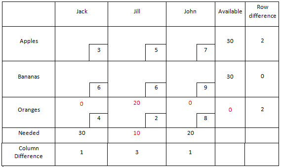
Now that the table is set up, we can begin solving. First, we find the highest value from the row and column differences. For this example, the highest value is $3 in Jill’s column (Note; if there were multiple of the highest value, choosing the starting one is arbitrary). Using that column, we go to the row with the lowest cost, and assign as much of that item to her as we can. So for Jill, we assign her 20 pounds of oranges, and that is the most we can ship of oranges. This leaves no oranges available for anyone else (we can assign Jack and John zero oranges), and Jill now only needs 10 more pounds of fruit. We indicate these changes on the table in red:
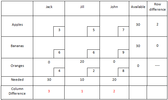
We can now consider the oranges row ‘done’. The next step is to reassign row and column difference values ignoring the costs in the oranges row. As no changes were made to the apples or bananas rows, their row difference values remain unchanged. However, the column differences are different. The differences become $6-$3 = $3 for Jack, $6-$5 = $1 for Jill, and $9-$7 = $2 for John. The changed values are marked in red in the table:
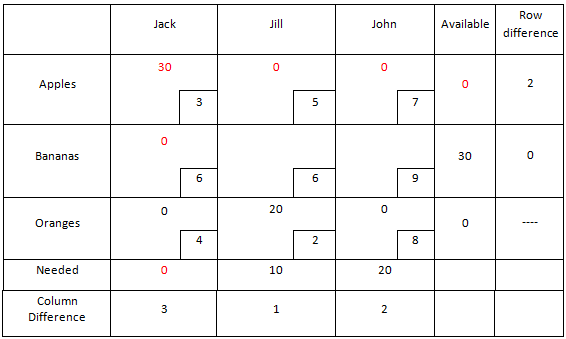
We repeat the fruit assignment step, giving as much fruit as constraints allow to the smallest cost in the row/column of the highest difference value. In this case, Jack gets 30 lbs of apples, which is all the fruit he needs and all the apples available. We mark the necessary changes to the table in red:
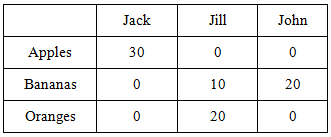
After this assignment, there are only two boxes (Jill-bananas and John-bananas) without assigned values. This allows us to do our final assignment without calculating row and column differences. We simply assign as much as we can to the cheapest option, then the remainder to the other. Of the remaining 30 lbs of bananas, Jill gets 10 lbs, bringing her needed fruit to zero and leaving 20 lbs of bananas for John, bringing his needed fruit to zero. The final assignment is as follows:
We find the total cost by taking the pounds of each fruit each person gets times the per unit cost of transporting that fruit to that person. Total cost = ($3*30 + $5*0 + $7*0 ) + ($6*0 + $6*10 + $9*20) + ($4*0 + $2*20 + $8*0) = $370. The Vogel Approximation Method often produces the optimal solution. Examining our solution for this example, we can see that changing the amounts of fruits anyone gets would lead to a higher cost, and thus our solution is optimal.
Conclusion
The transportation problem is a very special case when it comes to linear programming. As seen above, these problems can be time-consuming and very easy to make computational areas in, so in real-life applications, they would most likely be done by a computer. While initially the transportation problem was developed to solve problems in transporting goods from one the source to the destination, the transportation method can be used to solve other problems, such as what is referred to as an assignment problem. The assignment problem deals with the same concept but instead of transporting goods, it is used to assign people to jobs, machines, etc. Another application of the transportation problem is it can be used for things like scheduling as well. The only constraint in non-transporting problems is you have to be able to set up it up as a transportation matrix, or else there would be no way to solving the problem.
References
Dwyer, Paul S. The Direct Solution of the Transportation Problem with Reduced Matrices 13.1 (1966): 77-96. Institute for Operations Research and the Management Sciences. Web. Apr. 2016.
Havelick, Jaroslav, and Ludmila Domeova. "The Transportation Problem." Distance Learning Module for Management Science. N.p., n.d. Web. 21 Apr. 2016.
Reeb, James E., and Scott A. Leavengood. Transportation Problem: A Special Case for Linear Programming Problems. Corvallis, Or.: Oregon State U Extension Service, 2002. Web. Apr. 2016.
"Transportation Problem in Excel." Easy Excel Tutorial. Excel Easy, 2010. Web. 24 Apr. 2016.
Trick, Michael A. "Transportation Problem." Transportation Problem. N.p., 24 Aug. 1998. Web. 24 Apr. 2016.

