| (22 intermediate revisions by 3 users not shown) | |||
| Line 1: | Line 1: | ||
<br> | <br> | ||
| − | <center | + | <center> |
<font size="4">Downsampling </font> | <font size="4">Downsampling </font> | ||
| Line 8: | Line 8: | ||
</center> | </center> | ||
---- | ---- | ||
| + | ---- | ||
| + | <br> | ||
| − | + | == <font size="3"></font><font size="3"></font>Outline == | |
| − | + | ||
| − | + | ||
| − | + | ||
| − | <font size="3"></font> | + | |
| − | + | ||
| − | <font size="3"></font> | + | |
| − | + | ||
| − | + | ||
| − | + | ||
| − | + | ||
| − | + | ||
| − | + | ||
| − | + | ||
| − | + | ||
| − | + | ||
| − | + | ||
| − | + | ||
| − | + | ||
| − | + | ||
| − | + | ||
| − | + | ||
| − | + | ||
| − | + | ||
| − | + | ||
| − | + | ||
| − | + | ||
| − | + | ||
| − | + | ||
| − | + | ||
| − | + | ||
| − | + | ||
| − | + | ||
| − | + | ||
| − | + | ||
| − | + | ||
| − | + | ||
| − | + | ||
| − | + | ||
| − | + | ||
| − | + | ||
<font size="3"></font> | <font size="3"></font> | ||
| Line 76: | Line 38: | ||
<font size="3"> | <font size="3"> | ||
| − | |||
| − | |||
#Introduction | #Introduction | ||
#Definition of Downsampling<br> | #Definition of Downsampling<br> | ||
#Derivation of DTFT of downsampled signal<br> | #Derivation of DTFT of downsampled signal<br> | ||
#Example | #Example | ||
| − | # | + | #Decimator |
| − | # | + | #Conclusion<br> |
---- | ---- | ||
| Line 89: | Line 49: | ||
== Introduction == | == Introduction == | ||
| − | This slecture provides definition of downsampling, derives DTFT downsampled signal and demonstrates it in a frequency domain. Also, it explains process of decimation and why it needs a low-pass filter. | + | This slecture provides definition of downsampling, derives DTFT of downsampled signal and demonstrates it in a frequency domain. Also, it explains process of decimation and why it needs a low-pass filter. |
---- | ---- | ||
| Line 97: | Line 57: | ||
Downsampling is an operation which involves throwing away samples from discrete-time signal. Let ''x[n]'' be a digital-time signal shown below: <br> | Downsampling is an operation which involves throwing away samples from discrete-time signal. Let ''x[n]'' be a digital-time signal shown below: <br> | ||
| − | + | [[Image:Xofn.jpg]]<br> | |
then y[n] will be produced by downsampling ''x [n]'' by factor ''D'' = 3. So, ''y [n] = x[Dn]''. | then y[n] will be produced by downsampling ''x [n]'' by factor ''D'' = 3. So, ''y [n] = x[Dn]''. | ||
| − | + | [[Image:Yofn.jpg]]<br> | |
As seen in above graph, ''y [n]'' is obtained by throwing away some samples from x [n]. So, ''y [n]'' is a downsampled signal from | As seen in above graph, ''y [n]'' is obtained by throwing away some samples from x [n]. So, ''y [n]'' is a downsampled signal from | ||
| Line 134: | Line 94: | ||
<math>s_D [m]=\left\{ \begin{array}{ll} | <math>s_D [m]=\left\{ \begin{array}{ll} | ||
| − | 1,& \text{ if } n \text{ is a multiple of } | + | 1,& \text{ if } n \text{ is a multiple of } D,\\ |
0, & \text{ else}. | 0, & \text{ else}. | ||
\end{array}\right. = {\frac{1}{D}} \sum_{k = -\infty}^{D-1} e^{jk {\frac{2 \pi}{D} m}}</math> | \end{array}\right. = {\frac{1}{D}} \sum_{k = -\infty}^{D-1} e^{jk {\frac{2 \pi}{D} m}}</math> | ||
| Line 158: | Line 118: | ||
<br> | <br> | ||
| − | <br> | + | From two graphs it is seen that signal is stretched by D in frequency domain and decreased by D in a magnitude after downsampling. Both signals have the frequency of <math>\begin{align} |
| + | 2\pi | ||
| + | \end{align}</math> . | ||
| + | |||
| + | == Decimator == | ||
| + | |||
| + | As seen in second graph, if <math>\begin{align} | ||
| + | D2\pi T_1f_{max} | ||
| + | \end{align}</math> is greater than <math>\begin{align} | ||
| + | \pi | ||
| + | \end{align}</math> aliasing occurs. Downsampler is a part of a decimator which also has a low-pass filter to prevent aliasing. LPF eliminates signal components which has frequencies higher than cutoff frequency, which can be found from graphs shown above.<br> | ||
| + | |||
| + | <math>\begin{align} | ||
| + | & D\omega_c = D 2 \pi T_1 f_{max} < \pi\\ | ||
| + | & {\frac{T_2}{T_1}} 2\pi T_1 f_{max} < \pi \\ | ||
| + | & 2\pi T_2f_{max} < \pi \\ | ||
| + | &f_{max} < {\frac{1}{2T_2}} | ||
| + | \end{align}</math> | ||
| + | |||
| + | Thereby, signal needs to be filtered before downsampling if f<sub>max</sub> > 1/(2T<sub>2</sub>) . Complete block diagram of a decimator is shown below:<br> | ||
<br> | <br> | ||
| − | + | [[Image:Decimator cutoff.jpg]] | |
| − | + | <br> | |
| − | < | + | <br> |
| − | + | ---- | |
| − | + | == Conclusion == | |
| + | </font> | ||
| − | + | <font size="3"></font> | |
| − | + | <font size="3"></font> | |
| − | < | + | <font size="3"></font> |
| − | + | ||
| − | + | ||
| − | + | ||
| − | + | ||
| − | + | ||
| − | + | ||
| − | < | + | <font size="3"></font> |
| − | < | + | <font size="3"></font> |
| − | + | <font size="3"></font> | |
| − | = | + | <font size="3"></font> |
| − | + | <font size="3"></font> | |
| − | + | <font size="3"></font> | |
| − | + | <font size="3"></font> | |
| − | + | <font size="3"></font> | |
| − | + | <font size="3"></font> | |
| − | < | + | <font size="3"></font> |
| − | + | <font size="3"></font> | |
| − | + | <font size="3"></font> | |
| − | + | <font size="3"></font> | |
| − | + | <font size="3"></font> | |
| − | = | + | <font size="3"></font> |
| − | </font> | + | |
<font size="3"></font> | <font size="3"></font> | ||
| Line 277: | Line 250: | ||
<font size="3"></font> | <font size="3"></font> | ||
| − | <font size="3"> | + | <font size="3"></font> |
| + | |||
| + | <font size="3">To summarize, downsampling is a process of removing samples from signal. After downsampling, signal decreases by factor D in the magnitude and stretches by D in frequency domain. In order to downsample a signal, it first should be filtered by LPF to prevent aliasing. Both LPF and downsampler are parts of a decimator. </font> | ||
<font size="3"></font> | <font size="3"></font> | ||
| Line 283: | Line 258: | ||
---- | ---- | ||
| − | + | <br> | |
| − | + | ||
| − | + | ||
---- | ---- | ||
| Line 293: | Line 266: | ||
---- | ---- | ||
| − | == [[ | + | == [[Yeshmukhanbetov ECE438 slecture review|Questions and comments]] == |
| − | If you have any questions, comments, etc. please post them on [[ | + | If you have any questions, comments, etc. please post them on [[Yeshmukhanbetov ECE438 slecture review|this page]]. |
---- | ---- | ||
| − | + | [[2014_Fall_ECE_438_Boutin_digital_signal_processing_slectures|Back to ECE438 slectures, Fall 2014]] | |
| − | [[ | + | |
[[Category:Slecture]] [[Category:ECE438Fall2014Boutin]] [[Category:ECE]] [[Category:ECE438]] [[Category:Signal_processing]] | [[Category:Slecture]] [[Category:ECE438Fall2014Boutin]] [[Category:ECE]] [[Category:ECE438]] [[Category:Signal_processing]] | ||
Latest revision as of 18:07, 16 March 2015
Downsampling
A slecture by ECE student Yerkebulan Yeshmukhanbetov
Partly based on the ECE438 Fall 2014 lecture material of Prof. Mireille Boutin.
Contents
Outline
- Introduction
- Definition of Downsampling
- Derivation of DTFT of downsampled signal
- Example
- Decimator
- Conclusion
Introduction
This slecture provides definition of downsampling, derives DTFT of downsampled signal and demonstrates it in a frequency domain. Also, it explains process of decimation and why it needs a low-pass filter.
Definition of Downsampling
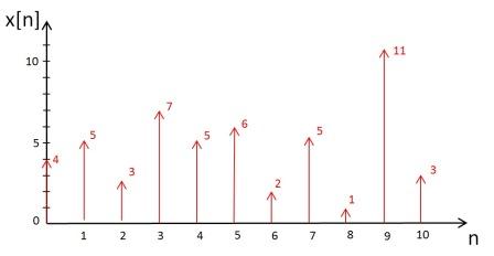
Downsampling is an operation which involves throwing away samples from discrete-time signal. Let x[n] be a digital-time signal shown below:
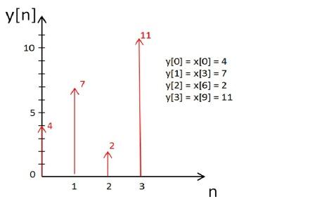
then y[n] will be produced by downsampling x [n] by factor D = 3. So, y [n] = x[Dn].
As seen in above graph, y [n] is obtained by throwing away some samples from x [n]. So, y [n] is a downsampled signal from
x [n].
Derivation of DTFT of downsampled signal
Let x (t) be a continuous time signal. Then x1 [n] = x (T1n) and x2 [n] = x (T2n). And ratio of sampling periods would be
D = T2/T1, which is an integer greater than 1. From these equations we obtain realtionship between x1 [n] and x2 [n].
$ \begin{align} x_2 [n] = x(T_2 n) = x(DT_1 n) = x_1 [nD] \end{align} $
Below we derive Discrete-Time Fourier Transform of x2 [n] in terms of DTFT of x1 [n].
$ \begin{align} &\mathcal{X}_2(\omega)= \mathcal{F}(x_2 [n]) = \mathcal{F}(x_1 [Dn])\\ &= \sum_{n = -\infty}^\infty x_1[Dn] e^{-j \omega n} = \sum_{m = -\infty}^\infty x_1[m] e^{-j \omega {\frac{m}{D}}}\\ &= \sum_{n = -\infty}^\infty s_D[m]* x_1 [m] e^{-j \omega {\frac{m}{D}}}\\ \end{align} $
where
$ s_D [m]=\left\{ \begin{array}{ll} 1,& \text{ if } n \text{ is a multiple of } D,\\ 0, & \text{ else}. \end{array}\right. = {\frac{1}{D}} \sum_{k = -\infty}^{D-1} e^{jk {\frac{2 \pi}{D} m}} $
$ \begin{align} &\mathcal{X}_2(\omega)= \sum_{m = -\infty}^\infty {\frac{1}{D}} \sum_{k = -\infty}^{D-1} e^{jk {\frac{2 \pi}{D} m}} x_1[m] e^{-j \omega {\frac{m}{D}}}\\ &= {\frac{1}{D}} \sum_{k = -\infty}^{D-1} \sum_{m = -\infty}^\infty x_1[m] e^{-jm ({\frac{\omega - 2 \pi k}{D}})} = \\ &= {\frac{1}{D}} \sum_{k = -\infty}^{D-1} \mathcal{X}_1 ({\frac{\omega - 2 \pi k}{D}}) \\ \end{align} $
Example
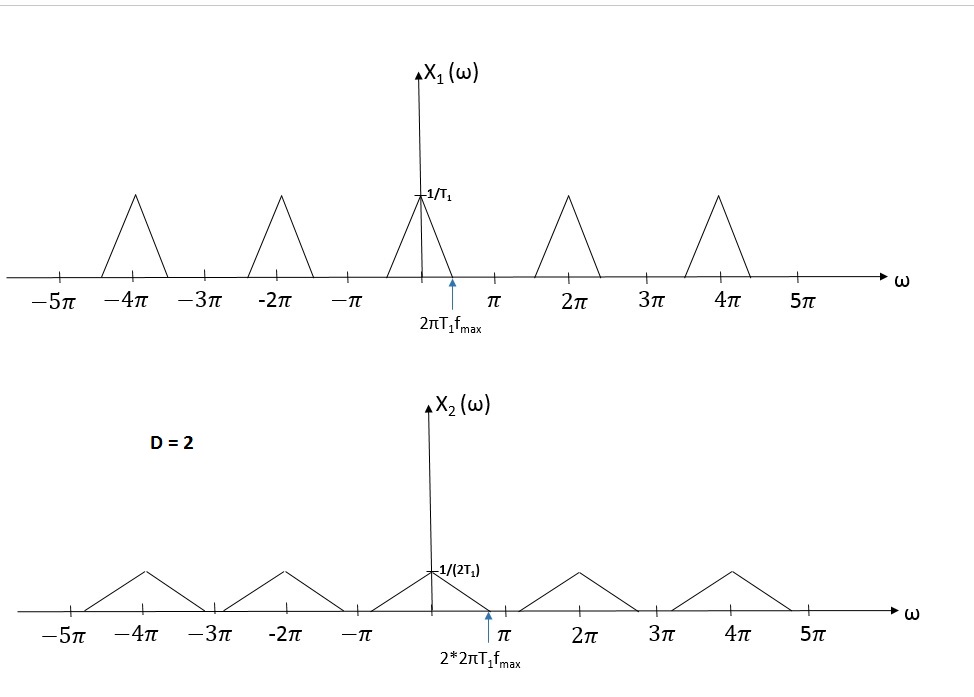
Let's take a look at an original signal X1 (w) and X2 (w) which is obtained after downsampling X1(w) by factor D = 2 in a frequency domain.
From two graphs it is seen that signal is stretched by D in frequency domain and decreased by D in a magnitude after downsampling. Both signals have the frequency of $ \begin{align} 2\pi \end{align} $ .
Decimator
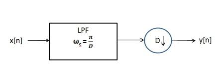
As seen in second graph, if $ \begin{align} D2\pi T_1f_{max} \end{align} $ is greater than $ \begin{align} \pi \end{align} $ aliasing occurs. Downsampler is a part of a decimator which also has a low-pass filter to prevent aliasing. LPF eliminates signal components which has frequencies higher than cutoff frequency, which can be found from graphs shown above.
$ \begin{align} & D\omega_c = D 2 \pi T_1 f_{max} < \pi\\ & {\frac{T_2}{T_1}} 2\pi T_1 f_{max} < \pi \\ & 2\pi T_2f_{max} < \pi \\ &f_{max} < {\frac{1}{2T_2}} \end{align} $
Thereby, signal needs to be filtered before downsampling if fmax > 1/(2T2) . Complete block diagram of a decimator is shown below:
Conclusion
To summarize, downsampling is a process of removing samples from signal. After downsampling, signal decreases by factor D in the magnitude and stretches by D in frequency domain. In order to downsample a signal, it first should be filtered by LPF to prevent aliasing. Both LPF and downsampler are parts of a decimator.
Questions and comments
If you have any questions, comments, etc. please post them on this page.


