| (39 intermediate revisions by 2 users not shown) | |||
| Line 24: | Line 24: | ||
==Introduction== | ==Introduction== | ||
| − | This Slecture will look into the relationship between a signal and the sampling of that signal in the view of the frequency domain. The signal that will be sampled will be in the time domain <math> x(t) </math>and after it was Fourier transformed, the sampled signal <math> X(f) </math> will be in the frequency domain. Here, we will see the relationship between this two signals and what rules need to be obeyed in order to create a good sampling signal. | + | This Slecture will look into the relationship between a signal and the sampling of that signal in the view of the frequency domain. The signal that will be sampled will be in the time domain <math> x(t) </math> and after it was Fourier transformed, the sampled signal <math> X(f) </math> will be in the frequency domain. Here, we will see the relationship between this two signals and what rules need to be obeyed in order to create a good sampling signal within the frequency domain. |
---- | ---- | ||
| + | |||
| + | ==Main Points== | ||
| + | |||
| + | *The sampling of a signal in the time domain <math> x(t) </math> is basically the repetition of the sampled signal <math> x(t) </math> or the <math> rep </math> function in the frequency domain. The graphical interpretation for this relationship can be seen in the picture below | ||
| + | |||
| + | [[Image:Sl1.jpg|500px|relationship view for the sampling signal between time domain and frequency domain]] | ||
| + | |||
| + | *From the picture above, I should point out that this relationship goes both ways, if we try to sample a signal from the frequency domain the sampled signal that will be produced in the time domain will also be in the form a of <math> rep </math> function. | ||
| + | |||
| + | *When we sampled a signal in the time domain, we usually sample a continuous time signal. However, we can't just sample the signal without discreeting the points within the continuous time signal. The reason for this is because, each discreet points within the continuous time signal will be the sampled points of the sampled signal in the frequency domain. The graphical interpretation for this relationship can be seen in the picture below | ||
| + | |||
| + | [[Image:Sl2.jpg|500px|relationship view for the sampling signal between time domain and frequency domain]] | ||
| + | |||
| + | *We should now look at some of the important facts of a sampled signal. One of the key factor in sampling a signal is to avoid the aliasing effect when sampling. Aliasing effect is when two sampled signals overlap (at least some part of it) with one another. This will produce distortions within a sampled signal. In order for us to avoid aliasing effect, we need to have a sampling frequency which is larger than two times the cut-offs frequencies. This is known as the Nyquist Theorem: | ||
| + | |||
| + | <div style="margin-left: 3em;"> | ||
| + | <math> | ||
| + | \begin{align} | ||
| + | f_s > 2 \times f_c\\ | ||
| + | \end{align} | ||
| + | </math> | ||
| + | </div> | ||
| + | <font size> | ||
| + | |||
| + | *The Nyquist theorem can be depicted through the graphical interpretation which can be seen through the picture below | ||
| + | |||
| + | [[Image:Sl_3a.jpg|500px|Graphical interpretation of Nyquist theorem]] | ||
| + | [[Image:Sl_3b.jpg|500px|Graphical interpretation of Nyquist theorem]] | ||
| + | |||
| + | *Now that we have looked at the graphical interpretation of sampling, we should next see the analytical expression of sampling in the view of the frequency domain. The Fourier transform of sampling is given by: | ||
| + | |||
| + | <div style="margin-left: 3em;"> | ||
| + | <math> | ||
| + | \begin{align} | ||
| + | X_s(f) &= S_t(f) * X(f)\\ | ||
| + | \end{align} | ||
| + | </math> | ||
| + | </div> | ||
| + | <font size> | ||
| + | |||
| + | *Since:- | ||
| + | |||
| + | <div style="margin-left: 3em;"> | ||
| + | <math> | ||
| + | \begin{align} | ||
| + | s_t(f) &= rep_T(\frac{1}{tau}rect(\frac{t}{tau}))\\ | ||
| + | \end{align} | ||
| + | </math> | ||
| + | </div> | ||
| + | <font size> | ||
| + | |||
| + | *Thus: | ||
| + | |||
| + | <div style="margin-left: 3em;"> | ||
| + | <math> | ||
| + | \begin{align} | ||
| + | S_t(f) &=\frac{1}{T}comb_\frac{1}{T}(sinc(tau + 1))\\ | ||
| + | &= \frac{1}{T}\sum_{k = -\infty}^\infty sinc(tauK/T) \delta(f-\frac{k}{T})\\ | ||
| + | \end{align} | ||
| + | </math> | ||
| + | </div> | ||
| + | <font size> | ||
| + | |||
| + | *Therefore: | ||
| + | |||
| + | <div style="margin-left: 3em;"> | ||
| + | <math> | ||
| + | \begin{align} | ||
| + | X_s(f) &= \frac{1}{T}\sum_{k = -\infty}^\infty sinc(tauK/T) \delta(f-\frac{k}{T}) * X(f)\\ | ||
| + | &= \frac{1}{T}\sum_{k = -\infty}^\infty sinc(tauK/T)X(f - \frac{k}{T})\\ | ||
| + | \end{align} | ||
| + | </math> | ||
| + | </div> | ||
| + | <font size> | ||
| + | |||
| + | *From the expression above we can see that the sampled signal is equal to the summation of the sinc function multiplied by the original signal which we wish to sampled and finally divided by the sampling period T. | ||
| + | ---- | ||
| + | |||
| + | ==Conclusion== | ||
| + | To conclude, in order to have a good sampling signal in the frequency domain, the sampling frequency must be at least twice the cut-off frequency. This theorem is known to be as the Nyquist theorem. If this theorem is obeyed, no aliasing would occur on the sampled signals and aliasing would occur if otherwise. Other than that, the sampling signal in the frequency domain is summation of the sinc function multiplied with the original signal which will later be divided by the sampling period T. | ||
| + | ---- | ||
| + | |||
| + | ==References== | ||
| + | [1].Mireille Boutin, "ECE438 Digital Signal Processing with Applications," Purdue University August 26,2009 | ||
| + | ---- | ||
| + | |||
| + | ==Questions and comments== | ||
| + | |||
| + | If you have any questions, comments, etc. please post them on [[Slecture_Topic7_Questions|this page]]. | ||
| + | ---- | ||
| + | [[2014_Fall_ECE_438_Boutin_digital_signal_processing_slectures|Back to ECE438 slectures, Fall 2014]] | ||
Latest revision as of 08:58, 14 March 2015
Frequency domain view of the relationship between a signal and a sampling of that signal
A slecture by ECE student Talha Takleh Omar Takleh
Partly based on the ECE438 Fall 2014 lecture material of Prof. Mireille Boutin.
Outline
- Introduction
- Main Points
- Conclusion
Introduction
This Slecture will look into the relationship between a signal and the sampling of that signal in the view of the frequency domain. The signal that will be sampled will be in the time domain $ x(t) $ and after it was Fourier transformed, the sampled signal $ X(f) $ will be in the frequency domain. Here, we will see the relationship between this two signals and what rules need to be obeyed in order to create a good sampling signal within the frequency domain.
Main Points
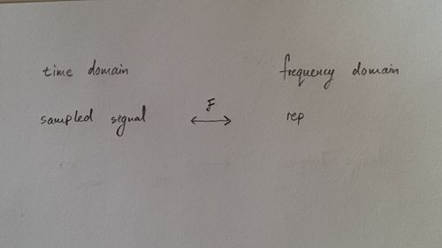
- The sampling of a signal in the time domain $ x(t) $ is basically the repetition of the sampled signal $ x(t) $ or the $ rep $ function in the frequency domain. The graphical interpretation for this relationship can be seen in the picture below
- From the picture above, I should point out that this relationship goes both ways, if we try to sample a signal from the frequency domain the sampled signal that will be produced in the time domain will also be in the form a of $ rep $ function.
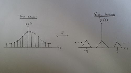
- When we sampled a signal in the time domain, we usually sample a continuous time signal. However, we can't just sample the signal without discreeting the points within the continuous time signal. The reason for this is because, each discreet points within the continuous time signal will be the sampled points of the sampled signal in the frequency domain. The graphical interpretation for this relationship can be seen in the picture below
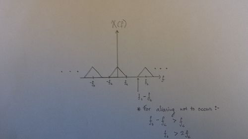
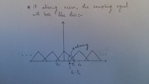
- We should now look at some of the important facts of a sampled signal. One of the key factor in sampling a signal is to avoid the aliasing effect when sampling. Aliasing effect is when two sampled signals overlap (at least some part of it) with one another. This will produce distortions within a sampled signal. In order for us to avoid aliasing effect, we need to have a sampling frequency which is larger than two times the cut-offs frequencies. This is known as the Nyquist Theorem:
$ \begin{align} f_s > 2 \times f_c\\ \end{align} $
- The Nyquist theorem can be depicted through the graphical interpretation which can be seen through the picture below
- Now that we have looked at the graphical interpretation of sampling, we should next see the analytical expression of sampling in the view of the frequency domain. The Fourier transform of sampling is given by:
$ \begin{align} X_s(f) &= S_t(f) * X(f)\\ \end{align} $
- Since:-
$ \begin{align} s_t(f) &= rep_T(\frac{1}{tau}rect(\frac{t}{tau}))\\ \end{align} $
- Thus:
$ \begin{align} S_t(f) &=\frac{1}{T}comb_\frac{1}{T}(sinc(tau + 1))\\ &= \frac{1}{T}\sum_{k = -\infty}^\infty sinc(tauK/T) \delta(f-\frac{k}{T})\\ \end{align} $
- Therefore:
$ \begin{align} X_s(f) &= \frac{1}{T}\sum_{k = -\infty}^\infty sinc(tauK/T) \delta(f-\frac{k}{T}) * X(f)\\ &= \frac{1}{T}\sum_{k = -\infty}^\infty sinc(tauK/T)X(f - \frac{k}{T})\\ \end{align} $
- From the expression above we can see that the sampled signal is equal to the summation of the sinc function multiplied by the original signal which we wish to sampled and finally divided by the sampling period T.
Conclusion
To conclude, in order to have a good sampling signal in the frequency domain, the sampling frequency must be at least twice the cut-off frequency. This theorem is known to be as the Nyquist theorem. If this theorem is obeyed, no aliasing would occur on the sampled signals and aliasing would occur if otherwise. Other than that, the sampling signal in the frequency domain is summation of the sinc function multiplied with the original signal which will later be divided by the sampling period T.
References
[1].Mireille Boutin, "ECE438 Digital Signal Processing with Applications," Purdue University August 26,2009
Questions and comments
If you have any questions, comments, etc. please post them on this page.


