| (11 intermediate revisions by 3 users not shown) | |||
| Line 4: | Line 4: | ||
[[Category:ECE438]] | [[Category:ECE438]] | ||
[[Category:signal processing]] | [[Category:signal processing]] | ||
| + | [[Category:Discrete-time_Fourier_transform]] | ||
<center><font size= 4> | <center><font size= 4> | ||
| Line 14: | Line 15: | ||
</center> | </center> | ||
---- | ---- | ||
| + | ---- | ||
| + | |||
| + | <center><font size= 3> | ||
| + | Background | ||
| + | </font size></center> | ||
| + | |||
---- | ---- | ||
A cosine wave with frequency f can be written as <math>cos(2 \pi f t)</math>. When sampling this cosine with period T (frequency <math>f_{s}=1/T</math>, the sampled signal <math>x[n]</math> can be written as <math>x[n]=cos(\frac{2 \pi f n}{T})</math>. | A cosine wave with frequency f can be written as <math>cos(2 \pi f t)</math>. When sampling this cosine with period T (frequency <math>f_{s}=1/T</math>, the sampled signal <math>x[n]</math> can be written as <math>x[n]=cos(\frac{2 \pi f n}{T})</math>. | ||
| Line 24: | Line 31: | ||
In continuous time, the signal looks like this: | In continuous time, the signal looks like this: | ||
| − | [[Image: | + | <center>[[Image:srhfig1.png|signal]]</center> |
Using the continuous time signal, it is possible to sample the signal. Due to the Nyquist Theorem, <math>f_{s}>1760\ Hz</math>. To demonstrate sampling above the Nyquist Rate, a <math>f_{s}</math> of 2000 Hz will be used. The sampling points are shown in red on top of the original signal below | Using the continuous time signal, it is possible to sample the signal. Due to the Nyquist Theorem, <math>f_{s}>1760\ Hz</math>. To demonstrate sampling above the Nyquist Rate, a <math>f_{s}</math> of 2000 Hz will be used. The sampling points are shown in red on top of the original signal below | ||
| − | [[Image: | + | <center>[[Image:srhfig2.png|Sampling]]</center> |
| + | |||
| + | ---- | ||
| + | <center><font size= 3> | ||
| + | CTFT vs DTFT | ||
| + | </font size></center> | ||
In order to understand what is happening in the frequency domain, we can compare the CTFT of the cosine to the DTFT of the sampled cosine. | In order to understand what is happening in the frequency domain, we can compare the CTFT of the cosine to the DTFT of the sampled cosine. | ||
| Line 36: | Line 48: | ||
<math>X(f)=\frac{\delta(f-880)+\delta(f+880)}{2}</math> | <math>X(f)=\frac{\delta(f-880)+\delta(f+880)}{2}</math> | ||
| + | <center>[[Image:srhfig3.png|CTFT]]</center> | ||
| + | |||
| + | To obtain the DTFT from the CTFT, three steps must occur: | ||
| + | |||
| + | * Rescale the frequency axis: <math>\chi(\omega) = X(\frac{\omega f_{s}}{2 \pi })</math> | ||
| + | * Rescale the magnitude by 1/T | ||
| + | * Repeat ("rep") the signal every <math>2 \pi</math> | ||
| + | <center><font size= 3> | ||
| + | Sampling above the nyquist rate | ||
| + | </font size></center> | ||
| + | For the sampling at 2000Hz, this results in the following DTFT: | ||
| + | |||
| + | <math>\Chi(\omega)=2000\frac{\delta(\frac{2000 \omega}{2 \pi }-880)+\delta(\frac{2000 \omega}{2 \pi }+880)}{2}, -\pi<\omega<\pi</math> | ||
| + | |||
| + | <math>\Chi(\omega)=2000\frac{\delta(\frac{2000 \omega-2 \pi 880}{2 \pi })+\delta(\frac{2000 \omega+2 \pi 880}{2 \pi })}{2}, -\pi<\omega<\pi</math> | ||
| + | |||
| + | <math>\Chi(\omega)=2000\frac{\delta(2000\frac{ \omega-2 \pi \frac{880}{2000}}{2 \pi })+\delta(\frac{2000\omega+2 \pi \frac{880}{2000}}{2 \pi })}{2}, -\pi<\omega<\pi</math> | ||
| + | |||
| + | |||
| + | <math>\Chi(\omega)=2\pi \frac{\delta( \omega- \pi \frac{880}{1000})+\delta(\omega+\pi \frac{880}{1000})}{2}, -\pi<\omega<\pi</math> | ||
| + | |||
| + | <math>\Chi(\omega)=\pi \delta( \omega- \pi \frac{880}{1000})+\pi \delta(\omega+\pi \frac{880}{1000}), -\pi<\omega<\pi</math> | ||
| + | |||
| + | <math>\Chi(\omega)=\left\{\begin{array}{ll}\pi \delta( \omega- \pi \frac{880}{1000})+\pi \delta(\omega+\pi \frac{880}{1000}), & \text{ if }-\pi<\omega<\pi,\\ \text{periodic period } 2\pi\end{array} \right. \ </math> | ||
| + | |||
| + | [[Image:srhfig4.png|Sampling Above Nyquist]] | ||
| + | |||
| + | |||
| + | <center><font size= 3> | ||
| + | Sampling Below the Nyquist Rate | ||
| + | </font size></center> | ||
| + | |||
| + | We can repeat the same process for a sampling below the Nyquist rate. In this case, we will sample at 1000 Hz. Using the same process as above, the result is: | ||
| + | |||
| + | <math>\Chi(\omega)=\left\{\begin{array}{ll}\pi \delta( \omega- \pi \frac{880}{500})+\pi \delta(\omega+\pi \frac{880}{500}), & \ ,\\ \text{periodic period } 2\pi\end{array} \right. \ </math> | ||
| + | |||
| + | <math>\Chi(\omega)=\left\{\begin{array}{ll}\pi \delta( \omega- \pi \frac{120}{500})+\pi \delta(\omega+\pi \frac{120}{500}), & \text{ if }-\pi<\omega<\pi,\\ \text{periodic period } 2\pi\end{array} \right. \ </math> | ||
| + | |||
| + | The plot of the DTFT is shown below: | ||
| + | <center>[[Image:srhfig5.png|Sampling Below Nyquist]]</center> | ||
| + | Note that the original frequency components are outside of the <math>[-\pi,\pi]</math> range. This leads to aliasing, which creates an additional frequency component at 120 Hz. This illustrates the fact that sampling below the nyquist rate will create aliasing and prevent shannnon reconstruction of the signal. | ||
---- | ---- | ||
| + | <center><font size= 3> | ||
| + | Conclusion | ||
| + | </font size></center> | ||
| + | As a brief overview, there are two main takeaways: | ||
| + | *The DTFT can be obtained from the CTFT by time scaling f by <math>2\pi/f_s</math>, magnitude scaling by <math>f_s</math>, and repeating every <math>2\pi</math> | ||
| + | *Sampling below the nyquist rate will cause aliasing and add low frequency components to the signal, potentially preventing any recovery. | ||
---- | ---- | ||
---- | ---- | ||
| − | + | ==[[SRH_Slecture_Review|Questions and comments]]== | |
| − | ==[[ | + | |
| − | If you have any questions, comments, etc. please post them on [[ | + | If you have any questions, comments, etc. please post them on [[SRH_Slecture_Review|this page]]. |
---- | ---- | ||
| − | [[ | + | [[2014_Fall_ECE_438_Boutin_digital_signal_processing_slectures|Back to ECE438 slectures, Fall 2014]] |
Latest revision as of 19:04, 16 March 2015
Discrete-time Fourier transform (DTFT) of a sampled cosine
A slecture by ECE student Sutton Hathorn
Partly based on the ECE438 Fall 2014 lecture material of Prof. Mireille Boutin.
Background
A cosine wave with frequency f can be written as $ cos(2 \pi f t) $. When sampling this cosine with period T (frequency $ f_{s}=1/T $, the sampled signal $ x[n] $ can be written as $ x[n]=cos(\frac{2 \pi f n}{T}) $.
The nyquist rate for a given signal is given as $ f_{s} = 2 f_{m} $, where $ f_{m} $ is the highest frequency in the signal. Since a cosine has only one positive frequency, for a cosine $ f_{m}=f $ and the nyquist rate is $ f_{s}=2 f \ Hz $.
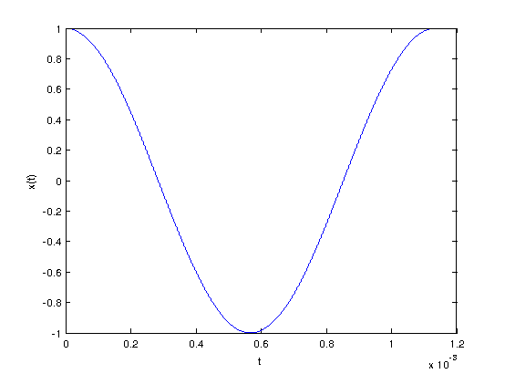
For demonstration, consider a cosine with frequency 880 Hz. This represents a pure A note. This signal can be written as: $ x(t)=cos(2 \pi 880 t) $
In continuous time, the signal looks like this:
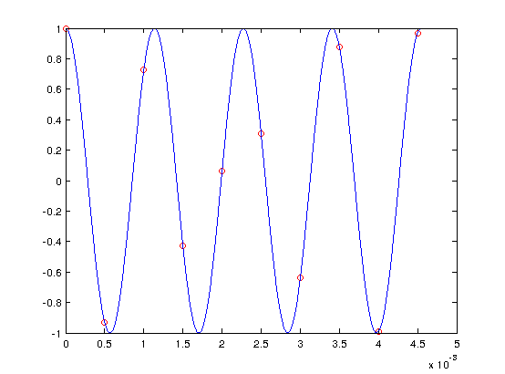
Using the continuous time signal, it is possible to sample the signal. Due to the Nyquist Theorem, $ f_{s}>1760\ Hz $. To demonstrate sampling above the Nyquist Rate, a $ f_{s} $ of 2000 Hz will be used. The sampling points are shown in red on top of the original signal below
CTFT vs DTFT
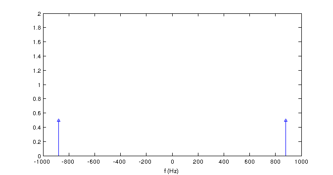
In order to understand what is happening in the frequency domain, we can compare the CTFT of the cosine to the DTFT of the sampled cosine.
From the CTFT table, the CTFT of a Cosine is
$ X(f)=\frac{\delta(f-880)+\delta(f+880)}{2} $
To obtain the DTFT from the CTFT, three steps must occur:
- Rescale the frequency axis: $ \chi(\omega) = X(\frac{\omega f_{s}}{2 \pi }) $
- Rescale the magnitude by 1/T
- Repeat ("rep") the signal every $ 2 \pi $
Sampling above the nyquist rate
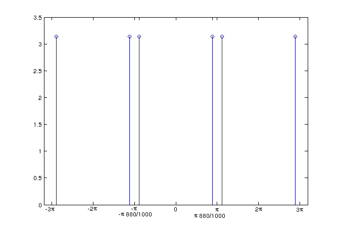
For the sampling at 2000Hz, this results in the following DTFT:
$ \Chi(\omega)=2000\frac{\delta(\frac{2000 \omega}{2 \pi }-880)+\delta(\frac{2000 \omega}{2 \pi }+880)}{2}, -\pi<\omega<\pi $
$ \Chi(\omega)=2000\frac{\delta(\frac{2000 \omega-2 \pi 880}{2 \pi })+\delta(\frac{2000 \omega+2 \pi 880}{2 \pi })}{2}, -\pi<\omega<\pi $
$ \Chi(\omega)=2000\frac{\delta(2000\frac{ \omega-2 \pi \frac{880}{2000}}{2 \pi })+\delta(\frac{2000\omega+2 \pi \frac{880}{2000}}{2 \pi })}{2}, -\pi<\omega<\pi $
$ \Chi(\omega)=2\pi \frac{\delta( \omega- \pi \frac{880}{1000})+\delta(\omega+\pi \frac{880}{1000})}{2}, -\pi<\omega<\pi $
$ \Chi(\omega)=\pi \delta( \omega- \pi \frac{880}{1000})+\pi \delta(\omega+\pi \frac{880}{1000}), -\pi<\omega<\pi $
$ \Chi(\omega)=\left\{\begin{array}{ll}\pi \delta( \omega- \pi \frac{880}{1000})+\pi \delta(\omega+\pi \frac{880}{1000}), & \text{ if }-\pi<\omega<\pi,\\ \text{periodic period } 2\pi\end{array} \right. \ $
Sampling Below the Nyquist Rate
We can repeat the same process for a sampling below the Nyquist rate. In this case, we will sample at 1000 Hz. Using the same process as above, the result is:
$ \Chi(\omega)=\left\{\begin{array}{ll}\pi \delta( \omega- \pi \frac{880}{500})+\pi \delta(\omega+\pi \frac{880}{500}), & \ ,\\ \text{periodic period } 2\pi\end{array} \right. \ $
$ \Chi(\omega)=\left\{\begin{array}{ll}\pi \delta( \omega- \pi \frac{120}{500})+\pi \delta(\omega+\pi \frac{120}{500}), & \text{ if }-\pi<\omega<\pi,\\ \text{periodic period } 2\pi\end{array} \right. \ $
The plot of the DTFT is shown below:
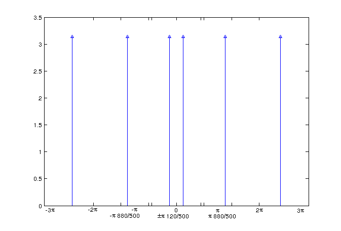
Note that the original frequency components are outside of the $ [-\pi,\pi] $ range. This leads to aliasing, which creates an additional frequency component at 120 Hz. This illustrates the fact that sampling below the nyquist rate will create aliasing and prevent shannnon reconstruction of the signal.
Conclusion
As a brief overview, there are two main takeaways:
- The DTFT can be obtained from the CTFT by time scaling f by $ 2\pi/f_s $, magnitude scaling by $ f_s $, and repeating every $ 2\pi $
- Sampling below the nyquist rate will cause aliasing and add low frequency components to the signal, potentially preventing any recovery.
Questions and comments
If you have any questions, comments, etc. please post them on this page.

