| (6 intermediate revisions by the same user not shown) | |||
| Line 1: | Line 1: | ||
| − | == A Solution Method For Zero-Dimensional Polynomial Equation System == | + | == A Solution Method For Zero-Dimensional Polynomial Equation System == |
'''Motivation''' | '''Motivation''' | ||
| Line 7: | Line 7: | ||
We first approximate the curve defined by the contour of the template object by an implicit polynomial equation. This yields a bivariate polynomial equation p(x,y) = 0 whose solution set approximates the template contour. | We first approximate the curve defined by the contour of the template object by an implicit polynomial equation. This yields a bivariate polynomial equation p(x,y) = 0 whose solution set approximates the template contour. | ||
| − | Let (x_i,y_i) , i=1, ..., N be the points of the point cloud. We are looking for the rotation R and the translation T such that p((xi, yi)R + T) = 0 for all i = 1, ..., N. | + | Let (x_i,y_i) , i=1, ..., N be the points of the point cloud. We are looking for the rotation R and the translation T such that p((xi, yi)R + T) = 0 for all i = 1, ..., N. Then we have an overdetermined polynomial equation system with noisy coefficient, which contains N equations and unknown variables R and T. We need to solve this overdetermined polynomial system. |
</div> <div style="width: 30%; float: right;"> | </div> <div style="width: 30%; float: right;"> | ||
[[Image:Butterfly model.jpg|250px]] | [[Image:Butterfly model.jpg|250px]] | ||
| − | </div> <div style="width: 100%; float: left;"></div> | + | </div> <div style="width: 100%; float: left;"></div> |
| + | '''Pipeline of the Solution Method''' [[Image:Schematic Rep.jpg|860px]] | ||
| − | ''' | + | '''Algorithm''' |
| − | + | ||
| − | + | Univariate Polynomial Equations: | |
| − | + | [[Image:Algorithm Univariate.jpg|900px]] | |
| − | + | Multivariate Polynomial Equations: | |
| − | + | [[Image:Algorithm Multivariate.jpg|900px]] | |
| − | [[Image: | + | '''Theorems''' |
| + | |||
| + | Univariate Polynomial Equations: | ||
| + | |||
| + | [[Image:Theorems1.png|650px]] | ||
| + | |||
| + | Multivariate Polynomial Equations: | ||
| + | |||
| + | [[Image:Theorems2.png|650px]] | ||
| + | |||
| + | '''Numerical Results''' | ||
| + | |||
| + | Picking 20 points along the contour of the butterfly and rotating and translating these 20 points using R = [0.6 -0.8; 0.8 0.6], and T = (-1, -1). Then registering the resulting 20 points back onto the original butterfly using the proposed method. | ||
| + | |||
| + | To demonstrate how the method allows us to deal with noisy observations of the template boundary, we added an increasing amount of Gaussian noise (with standard deviation between 0.01 and 0.2) to the x and y coordinates of the 20 points, repeating each experiment 10 times, and recorded the average Euclidean distance between the registered points and the original curve every time. The global match results and robustness analysis of the matches are plotted below. | ||
| + | |||
| + | [[Image:Butterflyfit.png|750px]] | ||
| + | |||
| + | To illustrate how the length of the curve being approximated by the point cloud affect the accuracy, we picked a segment of the butterfly contour curve and incrementally shrank the size of this contour. For each size increment, we picked 20 points on the curve segment and added Gaussian noise with standard deviation equal 0.05. Each experiment was repeated 10 times. The accuracy of the results, measured by the average Euclidean distance between the registered points and the butterfly contour, is plotted below. Some sample results are also given after that. One can see that the accuracy begins to degrade when the part of the curve being registered does not fit well with the implicit polynomial representation. | ||
| + | |||
| + | [[Image:Localmap.png|400px]] [[Image:Localsample.png|950px]] | ||
| + | |||
| + | '''References''' | ||
| + | |||
| + | [1] M. Boutin J. Zhang, S. Huang, Effective curve registration using a novel solution method for overdetermined systems of polynomial equations', In ''IS&T/SPIE joint symposium, Computational Imaging IV conference'', San Jose, CA, Jan. 2009. | ||
| + | |||
| + | [2] Ji Zhang, A solution method for zero dimensional polynomial equation systems and a pose-free framework for the robust solution of the structure from motion problem, ''Ph.D. Thesis'', Purdue University, Apr. 2009 | ||
Latest revision as of 06:14, 23 April 2010
A Solution Method For Zero-Dimensional Polynomial Equation System
Motivation
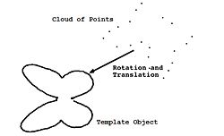
Consider the problem of curve registration, that is, finding the rotation and translation that best maps (i.e., registers) a cloud of points onto a template object, as described on the right.
We first approximate the curve defined by the contour of the template object by an implicit polynomial equation. This yields a bivariate polynomial equation p(x,y) = 0 whose solution set approximates the template contour.
Let (x_i,y_i) , i=1, ..., N be the points of the point cloud. We are looking for the rotation R and the translation T such that p((xi, yi)R + T) = 0 for all i = 1, ..., N. Then we have an overdetermined polynomial equation system with noisy coefficient, which contains N equations and unknown variables R and T. We need to solve this overdetermined polynomial system.
Pipeline of the Solution Method 
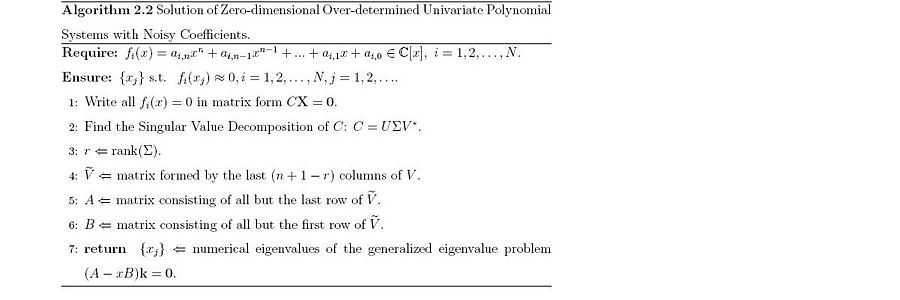
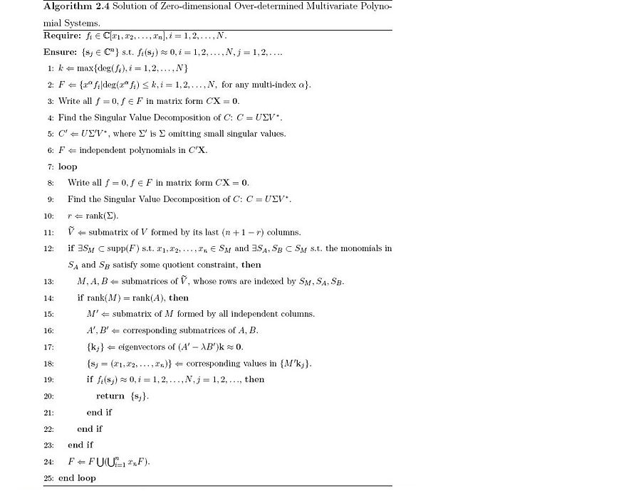
Algorithm
Univariate Polynomial Equations:
Multivariate Polynomial Equations:
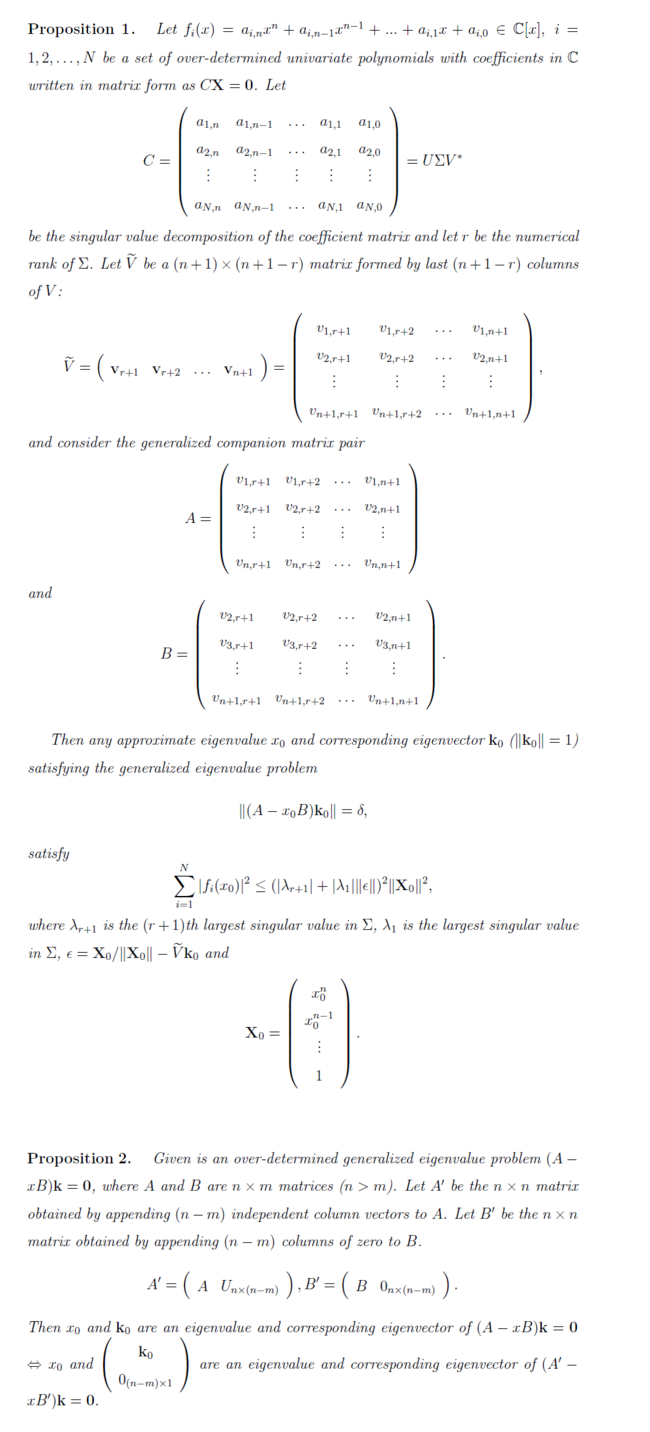
Theorems
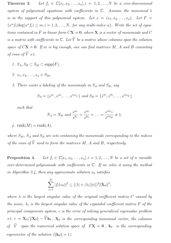
Univariate Polynomial Equations:
Multivariate Polynomial Equations:
Numerical Results
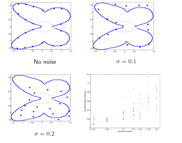
Picking 20 points along the contour of the butterfly and rotating and translating these 20 points using R = [0.6 -0.8; 0.8 0.6], and T = (-1, -1). Then registering the resulting 20 points back onto the original butterfly using the proposed method.
To demonstrate how the method allows us to deal with noisy observations of the template boundary, we added an increasing amount of Gaussian noise (with standard deviation between 0.01 and 0.2) to the x and y coordinates of the 20 points, repeating each experiment 10 times, and recorded the average Euclidean distance between the registered points and the original curve every time. The global match results and robustness analysis of the matches are plotted below.
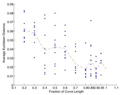
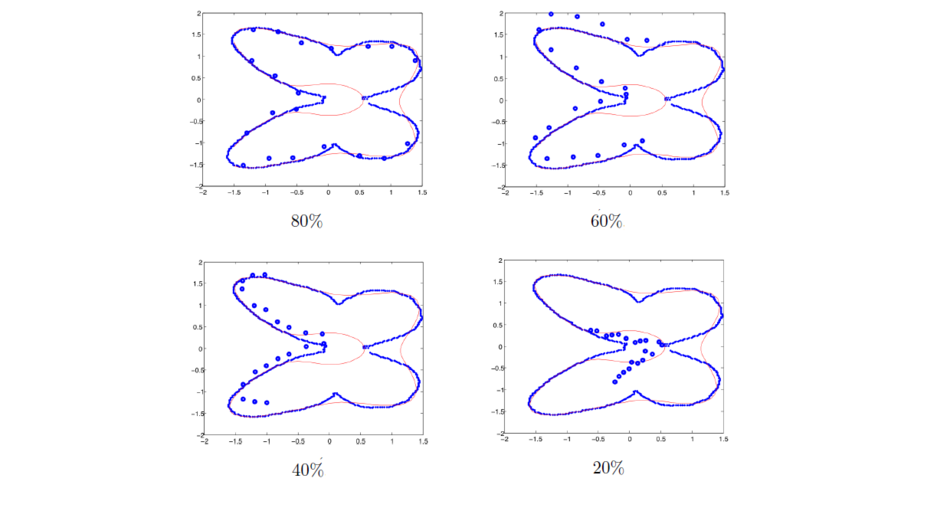
To illustrate how the length of the curve being approximated by the point cloud affect the accuracy, we picked a segment of the butterfly contour curve and incrementally shrank the size of this contour. For each size increment, we picked 20 points on the curve segment and added Gaussian noise with standard deviation equal 0.05. Each experiment was repeated 10 times. The accuracy of the results, measured by the average Euclidean distance between the registered points and the butterfly contour, is plotted below. Some sample results are also given after that. One can see that the accuracy begins to degrade when the part of the curve being registered does not fit well with the implicit polynomial representation.
References
[1] M. Boutin J. Zhang, S. Huang, Effective curve registration using a novel solution method for overdetermined systems of polynomial equations', In IS&T/SPIE joint symposium, Computational Imaging IV conference, San Jose, CA, Jan. 2009.
[2] Ji Zhang, A solution method for zero dimensional polynomial equation systems and a pose-free framework for the robust solution of the structure from motion problem, Ph.D. Thesis, Purdue University, Apr. 2009

