| (6 intermediate revisions by 2 users not shown) | |||
| Line 1: | Line 1: | ||
| − | + | [[Category:lecture notes]] | |
| + | [[Category:ECE438]] | ||
| + | [[Category:speech]] | ||
| + | ==Post Lecture Speech notes. [[ECE438]], Fall 2009, [[user:mboutin|Prof. Boutin]]== | ||
| + | (Click [[ECE438_(BoutinFall2009)|here]] to go to course wiki.) | ||
= Basic Idea = | = Basic Idea = | ||
* Speech is an acoustic signal, which we approximate as an analog signal. It is our goal to change this analog signal into a digital so that we can perform various forms of processing on it. | * Speech is an acoustic signal, which we approximate as an analog signal. It is our goal to change this analog signal into a digital so that we can perform various forms of processing on it. | ||
| Line 18: | Line 22: | ||
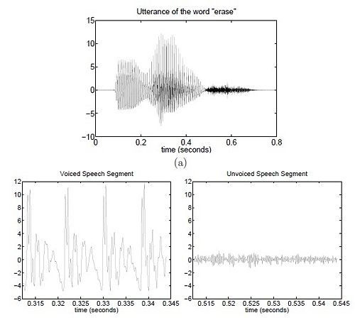
There are two methods to differentiate between the two when observing the time domain plot of the audio signal | There are two methods to differentiate between the two when observing the time domain plot of the audio signal | ||
| + | |||
| + | [[Image:VoicedvsUnvoiced.jpg|500px|Voiced and Unvoiced components of a voice signal]] | ||
1) Average Power: By comparing the average power <math>P = \frac{1}{L} \sum_{n=1}^L x^2(n)</math>. | 1) Average Power: By comparing the average power <math>P = \frac{1}{L} \sum_{n=1}^L x^2(n)</math>. | ||
| Line 23: | Line 29: | ||
2) Zero-crossings: Alternatively, you can compare how many times the signal crosses the zero-axis. | 2) Zero-crossings: Alternatively, you can compare how many times the signal crosses the zero-axis. | ||
| − | |||
| − | |||
* Zero crossing (Unvoiced) > Zero crossing (Voiced) | * Zero crossing (Unvoiced) > Zero crossing (Voiced) | ||
| + | |||
| + | Since the voiced section is approximately period, it can be modeled as a pulse train. Similarly, the unvoiced section can be modeled as white noise. | ||
= Modeling of Speech Production = | = Modeling of Speech Production = | ||
| Line 32: | Line 38: | ||
[[Image:Vocaltractmodel.jpg|500px|Model of Vocal tract]] | [[Image:Vocaltractmodel.jpg|500px|Model of Vocal tract]] | ||
| + | where <math>s(t) = x(t) \ast v(t)</math> where x(t) is the excitation (either pulse train or white noise) | ||
| + | |||
| + | = Modeling of the vocal tract = | ||
| + | I'm not going to go into extensive detail here (see class lecture notes) but I will go over the basics and the end result.. | ||
| + | |||
| + | Basically, the vocal tract is modeled as a finite series of connected tubes. | ||
| + | |||
| + | (u(t) is the signal going in the front of the tube, v(t) is the signal coming out of the front of the tube, w(t) is the signal coming out of the end of the tube, x(t) is the signal going into the end of the tube) | ||
| + | |||
| + | Using this model, we get two equations. | ||
| + | |||
| + | 1) Going through a tube: <math> | ||
| + | \begin{pmatrix} | ||
| + | U_d(z) \\ | ||
| + | V_d(z) | ||
| + | \end{pmatrix} | ||
| + | = z | ||
| + | \begin{pmatrix} | ||
| + | 1 & 0 \\ | ||
| + | 0 & z^{-2} | ||
| + | \end{pmatrix} | ||
| + | \begin{pmatrix} | ||
| + | W_d(z) \\ | ||
| + | X_d(z) | ||
| + | \end{pmatrix} | ||
| + | </math> | ||
| + | |||
| + | * This shows there is a time delay when traveling through a tube (the <math>z^(-2)</math> term) | ||
| + | |||
| + | 2) Between two tubes: <math> | ||
| + | \begin{pmatrix} | ||
| + | U_d(z) \\ | ||
| + | V_d(z) | ||
| + | \end{pmatrix} | ||
| + | = \frac{1}{1+r} | ||
| + | \begin{pmatrix} | ||
| + | A+B & A-B \\ | ||
| + | A-B & A+B | ||
| + | \end{pmatrix} | ||
| + | \begin{pmatrix} | ||
| + | W_d(z) \\ | ||
| + | X_d(z) | ||
| + | \end{pmatrix} | ||
| + | </math> | ||
| + | |||
| + | where r is a reflection coefficient <math>-1 <= r <= 1</math> such that <math>r = \frac{B-A}{B+A}</math> | ||
| + | |||
| + | The end result after modeling is a transfer function that is an all-pole filter with a gain and a time delay. | ||
| + | |||
| + | * Since the vocal tract is a cavity that resonates it makes sense that our output of a pulse train (voiced) convolved with a transfer function results in a series of varying-amplitude pulses with certain frequencies that are amplified. | ||
| + | * These frequencies are known as '''formants''' | ||
| + | |||
| + | = Transfer function = | ||
| + | As noted above, the transfer function is usually an all-pole filter. We can observe what the resonances, or formants, are just by looking at the function | ||
| + | * A real pole -> 1 formant | ||
| + | * A complex pole pair -> 1 formant | ||
| + | If you are instead given a z-model... | ||
| + | * <math>F = \frac{\theta}{2 \pi T} </math> , where F is the formant frequency and T is the sampling period. | ||
| + | |||
| + | Also, it should be noted that the transfer function is not always an all-pole filter. | ||
| + | * Zeros, or anti-resonances, will occur when there is no measurable output (i.e. Nasals and Fricatives) | ||
| + | ** Nasals => The output from the mouth is approximately 0 | ||
| + | ** Fricatives/stop consonants => blockage behind source is infinite (forcing air through a constriction) | ||
| + | |||
| + | = Spectrograms = | ||
| + | Since this was pretty well covered by both the lecture and lab, I'm just going to post a link to a site that I found helpful for further understanding how spectrograms work and how they tell us about different parts of speech. | ||
| + | |||
| + | -> How to read a spectrogram by Rob Hagiwara | ||
| + | http://home.cc.umanitoba.ca/~robh/howto.html | ||
prelecture notes here | prelecture notes here | ||
[[SupplementarySpeech_prelecture]] | [[SupplementarySpeech_prelecture]] | ||
| + | ---- | ||
| + | [[[[ECE438_(BoutinFall2009)|Back to ECE438, Fall 2009]] | ||
Latest revision as of 14:26, 10 April 2013
Contents
Post Lecture Speech notes. ECE438, Fall 2009, Prof. Boutin
(Click here to go to course wiki.)
Basic Idea
- Speech is an acoustic signal, which we approximate as an analog signal. It is our goal to change this analog signal into a digital so that we can perform various forms of processing on it.
Parts of Speech
- Before we jump into the mathematical "deep end" we first need to know the basic building blocks of speech
- A sentence that we hear is made up of syllables (sound) and separations (no sound). Simply put, a syllable is a single, uninterrupted sound that forms the rhythmical foundation of a language. For example, the word 'water' has two syllables, 'wa' and 'ter' separated by a tiny break in speech.
- If we go down further, each syllable is formed of phonemes. A phoneme is the smallest, segmental unit of sound. It is what forms the difference between utterances. Even though two different groups use the same language and have different accents and because the phonemes have the same function.
- Since phonemes are the smallest block of a speech signal, it is no surprise that they form the basis for speech analysis.
Phonemes
There are two types of phones, voiced and unvoiced.
- Voiced phonemes consist of all vowels and some consonants whereas unvoiced phonemes are just consonants.
There are two methods to differentiate between the two when observing the time domain plot of the audio signal
1) Average Power: By comparing the average power $ P = \frac{1}{L} \sum_{n=1}^L x^2(n) $.
- $ P_{avg,voiced} > P_{avg,unvoiced} $
2) Zero-crossings: Alternatively, you can compare how many times the signal crosses the zero-axis.
- Zero crossing (Unvoiced) > Zero crossing (Voiced)
Since the voiced section is approximately period, it can be modeled as a pulse train. Similarly, the unvoiced section can be modeled as white noise.
Modeling of Speech Production
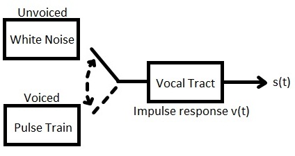
Utilizing this valuable information we can now construct a model for speech production as shown below.
where $ s(t) = x(t) \ast v(t) $ where x(t) is the excitation (either pulse train or white noise)
Modeling of the vocal tract
I'm not going to go into extensive detail here (see class lecture notes) but I will go over the basics and the end result..
Basically, the vocal tract is modeled as a finite series of connected tubes.
(u(t) is the signal going in the front of the tube, v(t) is the signal coming out of the front of the tube, w(t) is the signal coming out of the end of the tube, x(t) is the signal going into the end of the tube)
Using this model, we get two equations.
1) Going through a tube: $ \begin{pmatrix} U_d(z) \\ V_d(z) \end{pmatrix} = z \begin{pmatrix} 1 & 0 \\ 0 & z^{-2} \end{pmatrix} \begin{pmatrix} W_d(z) \\ X_d(z) \end{pmatrix} $
- This shows there is a time delay when traveling through a tube (the $ z^(-2) $ term)
2) Between two tubes: $ \begin{pmatrix} U_d(z) \\ V_d(z) \end{pmatrix} = \frac{1}{1+r} \begin{pmatrix} A+B & A-B \\ A-B & A+B \end{pmatrix} \begin{pmatrix} W_d(z) \\ X_d(z) \end{pmatrix} $
where r is a reflection coefficient $ -1 <= r <= 1 $ such that $ r = \frac{B-A}{B+A} $
The end result after modeling is a transfer function that is an all-pole filter with a gain and a time delay.
- Since the vocal tract is a cavity that resonates it makes sense that our output of a pulse train (voiced) convolved with a transfer function results in a series of varying-amplitude pulses with certain frequencies that are amplified.
- These frequencies are known as formants
Transfer function
As noted above, the transfer function is usually an all-pole filter. We can observe what the resonances, or formants, are just by looking at the function
- A real pole -> 1 formant
- A complex pole pair -> 1 formant
If you are instead given a z-model...
- $ F = \frac{\theta}{2 \pi T} $ , where F is the formant frequency and T is the sampling period.
Also, it should be noted that the transfer function is not always an all-pole filter.
- Zeros, or anti-resonances, will occur when there is no measurable output (i.e. Nasals and Fricatives)
- Nasals => The output from the mouth is approximately 0
- Fricatives/stop consonants => blockage behind source is infinite (forcing air through a constriction)
Spectrograms
Since this was pretty well covered by both the lecture and lab, I'm just going to post a link to a site that I found helpful for further understanding how spectrograms work and how they tell us about different parts of speech.
-> How to read a spectrogram by Rob Hagiwara
http://home.cc.umanitoba.ca/~robh/howto.html
prelecture notes here SupplementarySpeech_prelecture


