(→Code available) |
m |
||
| (12 intermediate revisions by 4 users not shown) | |||
| Line 1: | Line 1: | ||
| + | == Non-parametric techniques == | ||
| + | The non-parametric density estimation is | ||
| + | '''P(x) = k/(NV)''' | ||
| + | |||
| + | where, | ||
| + | *k is the number of samples in V | ||
| + | *N is the total number of samples | ||
| + | *V is the volume surrounding x | ||
| + | |||
| + | This estimate is computed by two approaches | ||
| + | |||
| + | '''Parzen window approach''' | ||
| + | *Fixing the volume V and determining the number k of data points inside V | ||
| + | |||
| + | '''KNN(K-Nearest Neighbor)''' | ||
| + | *Fixing the value of k and determining the minimum volume V that encompasses k points in the dataset | ||
| + | |||
| + | |||
| + | '''The advantages of non-parametric techniques''' | ||
| + | *No assumption about the distribution required ahead of time | ||
| + | *With enough samples we can converge to an target density | ||
| + | |||
| + | '''The disadvantages of non-parametric techniques''' | ||
| + | *If we have a good classification, the number of required samples may be very large | ||
| + | *Computationally expensive | ||
| + | |||
== k-Nearest Neighbor (kNN) Algorithm == | == k-Nearest Neighbor (kNN) Algorithm == | ||
| Line 38: | Line 64: | ||
== The Algorithm's pseudo-code == | == The Algorithm's pseudo-code == | ||
| − | Consider k as the desired number of nearest neighbors and S:={p_1, ... , p_n} be the set of training samples in the form p_1 = (x_i, c_i), where x_i is the d-dimensional feature vector of the point p_i and c_i is the class that p_i belongs to. | + | Consider k as the desired number of nearest neighbors and <math>S:={p_1, ... , p_n}</math> be the set of training samples in the form <math>p_1 = (x_i, c_i)</math>, where <math>x_i</math> is the d-dimensional feature vector of the point <math>p_i</math> and <math>c_i</math> is the class that <math>p_i</math> belongs to. |
For each p'=(x',c') | For each p'=(x',c') | ||
| Line 53: | Line 79: | ||
== References == | == References == | ||
| − | + | * "Introduction to Data Mining", P. Tan, M. Steinbach and V. Kumar, Addison-Wesley, 2006. | |
| + | |||
| + | * "Efficient Implementation of Nearest Neighbor Classification" [http://www.developer.com/java/article.php/10922_1491641_1] | ||
| − | + | * "Efficient Implementation of Nearest Neighbor Classification" (Slides) [http://people.ac.upc.edu/josepr/Talks/2005-05-23-CORES05-NN.pdf] | |
| − | - | + | * "k-Nearest Neighbors" (Wikipedia) <http://en.wikipedia.org/wiki/Nearest_neighbor_(pattern_recognition)> |
| − | + | [[Category:ECE662]] | |
Latest revision as of 07:46, 10 April 2008
Contents
Non-parametric techniques
The non-parametric density estimation is P(x) = k/(NV)
where,
- k is the number of samples in V
- N is the total number of samples
- V is the volume surrounding x
This estimate is computed by two approaches
Parzen window approach
- Fixing the volume V and determining the number k of data points inside V
KNN(K-Nearest Neighbor)
- Fixing the value of k and determining the minimum volume V that encompasses k points in the dataset
The advantages of non-parametric techniques
- No assumption about the distribution required ahead of time
- With enough samples we can converge to an target density
The disadvantages of non-parametric techniques
- If we have a good classification, the number of required samples may be very large
- Computationally expensive
k-Nearest Neighbor (kNN) Algorithm
This algorithm is based on the observation that a sample that has features that are similar to the ones of points of one particular class it belongs to that class. These points are known as nearest neighbors. The parameter k specifies the number of neighbors (neighboring points) used to classify one particular sample point. Finally, the assignment of a sample to a particular class is done by having the k neighbors considered to "vote". In this fashion, the class represented by the largest number of points among the neighbors ought to be the class that the sample belongs to. The so called Nearest Neighbor algorithm is the particular instance of the kNN when k=1.
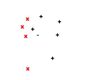
Consider the set of points in the feature space in the figure below:
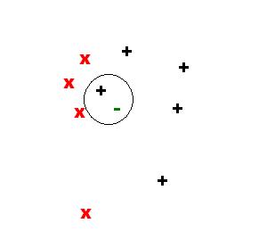
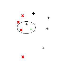
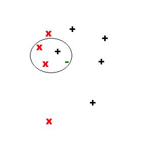
The next 3 figures illustrate the sample point in the feature space and neighbors for k={1,2,3}:
For k=1, we have:
For k=2, we have:
For k=3, we have:
Some of the important properties of the kNN algorithm are listed below:
- The kNN can be used to classify data without requiring model building, this is called "instance-based learning".
- A measurement of the distance between data points should be available
- The kNN classification is based solely on local information (only the k nearest neighboring data points are inspected during the classification process).
- The decision boundaries produced by the kNN classification can of of arbitrary shape
- The classification is sensitive to the correct selection of k. If k is too small it will lead to "over-fitting"
The Algorithm's pseudo-code
Consider k as the desired number of nearest neighbors and $ S:={p_1, ... , p_n} $ be the set of training samples in the form $ p_1 = (x_i, c_i) $, where $ x_i $ is the d-dimensional feature vector of the point $ p_i $ and $ c_i $ is the class that $ p_i $ belongs to.
For each p'=(x',c')
- Compute the distance $ d(x', x_i) $ between $ p' $ and all $ p_i $ belonging to S
- Sort all points $ p_i $ according to the key $ d(x',x_i) $
- Select the first $ k $ points from the sorted list, those are the $ k $ closest training samples to $ p' $
- Assign a class to $ p' $ based on majority vote: $ c' = argmax_y \sum_{(x_i,c_i)} $ belonging to S, $ I(y=c_i) $
end
Code available
- "Instance-Based learning Java Implementation" [1]
References
- "Introduction to Data Mining", P. Tan, M. Steinbach and V. Kumar, Addison-Wesley, 2006.
- "Efficient Implementation of Nearest Neighbor Classification" [2]
- "Efficient Implementation of Nearest Neighbor Classification" (Slides) [3]
- "k-Nearest Neighbors" (Wikipedia) <http://en.wikipedia.org/wiki/Nearest_neighbor_(pattern_recognition)>


