(New page: http://www.bigtennetwork.com/UserFiles/Image/Fan_pets/purdue_cat500.jpg) |
|||
| (3 intermediate revisions by the same user not shown) | |||
| Line 1: | Line 1: | ||
| + | In order to fully understand what this page is all about, you're going to need some basic understanding of what a periodic function is. To ensure you have this basic knowledge please revisist my earlier submissions for homework one, but a crash course can be found at the website listed below. | ||
| + | |||
http://www.bigtennetwork.com/UserFiles/Image/Fan_pets/purdue_cat500.jpg | http://www.bigtennetwork.com/UserFiles/Image/Fan_pets/purdue_cat500.jpg | ||
| + | |||
| + | Now, let's begin! | ||
| + | |||
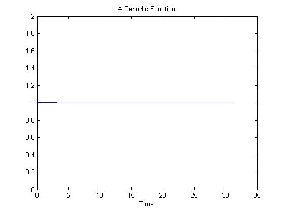
| + | 1. From sampling the values of a cosine function as described in the matlab code attached, the following periodic function, a simple line y = 1, was produced as figure 1 over the domain defined. | ||
| + | |||
| + | [[Image:Periodic_Function_Jack_ECE301Fall2008mboutin.jpg]] | ||
| + | |||
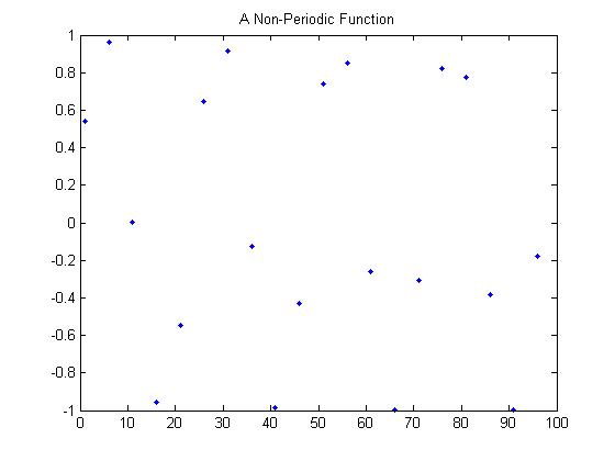
| + | An example of a non-periodic function derived from the same cosine function would be the scatter plot that the code generates in figure and can be seen below. | ||
| + | |||
| + | [[Image:Non_Periodic_Function_ECE301Fall2008mboutin.jpg]] | ||
| + | |||
| + | <pre> | ||
| + | %Jack Williams | ||
| + | %ECE 301 HW2 | ||
| + | %September 11th, 2008 | ||
| + | |||
| + | clear | ||
| + | clc | ||
| + | |||
| + | p = pi*[0 0.5 1 1.5 2 2.5 3 3.5 4 4.5 5 5.5 6 6.5 7 7.5 8 8.5 9 9.5 10]; | ||
| + | |||
| + | for i = 1:21 | ||
| + | for x = p(i) | ||
| + | y(i) = cos(x); | ||
| + | end | ||
| + | end | ||
| + | |||
| + | %Producing a periodic function, a straight horizontal line | ||
| + | %by sampling cosine values at whole period intervals | ||
| + | |||
| + | f=1; | ||
| + | |||
| + | for z = 1:4:21 | ||
| + | n(f) = y(z); | ||
| + | g(f) = p(z); | ||
| + | f = f + 1; | ||
| + | end | ||
| + | |||
| + | figure(1); | ||
| + | plot(g,n); | ||
| + | title('A Periodic Function'); | ||
| + | xlabel('Time'); | ||
| + | |||
| + | %Producing a non-periodic function by sampling cosine values | ||
| + | %at whole integer value intervals | ||
| + | |||
| + | e = 1; | ||
| + | |||
| + | for b = 1:5:100 | ||
| + | r(e) = cos(b); | ||
| + | s(e) = b; | ||
| + | e = e + 1; | ||
| + | end | ||
| + | |||
| + | r,s | ||
| + | |||
| + | figure(2); | ||
| + | plot(s,r,'.'); | ||
| + | title('A Non-Periodic Function') | ||
| + | </pre> | ||
Latest revision as of 15:14, 12 September 2008
In order to fully understand what this page is all about, you're going to need some basic understanding of what a periodic function is. To ensure you have this basic knowledge please revisist my earlier submissions for homework one, but a crash course can be found at the website listed below.

Now, let's begin!
1. From sampling the values of a cosine function as described in the matlab code attached, the following periodic function, a simple line y = 1, was produced as figure 1 over the domain defined.
An example of a non-periodic function derived from the same cosine function would be the scatter plot that the code generates in figure and can be seen below.
%Jack Williams
%ECE 301 HW2
%September 11th, 2008

clear
clc

p = pi*[0 0.5 1 1.5 2 2.5 3 3.5 4 4.5 5 5.5 6 6.5 7 7.5 8 8.5 9 9.5 10];

for i = 1:21
    for x = p(i)
        y(i) = cos(x);
    end
end

%Producing a periodic function, a straight horizontal line
%by sampling cosine values at whole period intervals

f=1;

for z = 1:4:21
    n(f) = y(z);
    g(f) = p(z);
    f = f + 1;
end

figure(1);
plot(g,n);
title('A Periodic Function');
xlabel('Time');

%Producing a non-periodic function by sampling cosine values
%at whole integer value intervals

e = 1;

for b = 1:5:100
    r(e) = cos(b);
    s(e) = b;
    e = e + 1;
end

r,s

figure(2);
plot(s,r,'.');
title('A Non-Periodic Function')


