m |
|||
| Line 171: | Line 171: | ||
[[File:BayesExample10.JPG]] | [[File:BayesExample10.JPG]] | ||
| − | + | TODO: Finish this section, include ethical part and how this data is not accurate. | |
Sources: | Sources: | ||
Revision as of 07:03, 28 November 2022
Probability : Group 4
Kalpit Patel Rick Jiang Bowen Wang Kyle Arrowood
Probability, Conditional Probability, Bayes Theorem Disease example
Definition: Probability is a measure of the likelihood of an event to occur. Many events cannot be predicted with total certainty. We can predict only the chance of an event to occur i.e., how likely they are going to happen, using it.
Notation:
1) Sample space (S): Set of all possible outcomes of an experiment (e.g., S={O1,O2,..,On}).
2) Event: Any subsets of outcomes (e.g., A={O1,O2,Ok}) contained in the sample space S.
Formula for probability:
1. Let N:= |S| be the size of sample space
2. Let N(A):= |A| be the number of simple outcomes contained in event A
3. Then P(A) = N(A)/N
Mutually exclusivity:
When events A and B have no outcomes in common ![]()
Axioms of probability:
1. Probability can range from 0 to 1, where 0 means the event to be an impossible one and 1 indicates a certain event. -> ![]()
2. The probability of all the events in a sample space adds up to 1. -> P(S) = 1
3. When all events have no outcomes in common.
-> ![]()
Conditional Probability:
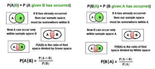
Conditional probability is defined as the likelihood of an event or outcome occurring, based on the occurrence of a previous event or outcome. It is the measure of the probability of an event E, given that another event F has already occurred. Some key points to note here are :
1. P(E|F): Here, E is the event whose probability we are calculating, and F is the event it is conditioned on.
2. "|": Is the symbol used to determine the unknown event (E) and the conditioning event (F).
3. P(F) > 0: The probability of the conditioning event must be positive, otherwise the conditional probability is undefined.
4. In essence, P(E|F) is basically the ratio of the intersection with the conditioning event, so we are measuring how much the conditioning event "influences" the possibility of another event.
Multiplication Rule:
If we rearrange the terms in our formula, we end up with P(E∩F) = P(E|F)P(F), which means the probability of the intersection of two events E and F can be calculated by the product of the conditional probability of one event given another and the probability of the conditioning event.
But what if we have multiple events which we want to condition? In other words, what if want to find how much the likelihood of a particular event is influenced or altered by the occurrence of more than 1 events, say "N" events namely: E1, E2,....,En.
This is called the multiplication rule of probability, and is extremely useful in finding the probability of multiple events occurring together.
Independent Events:
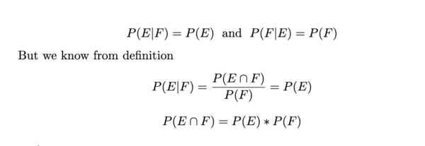
This is a special case of Conditional Probability, where the occurrence of one event does not affect the probability of another event. In other words, for two events E and F:
Baye's Theorem Derivation:
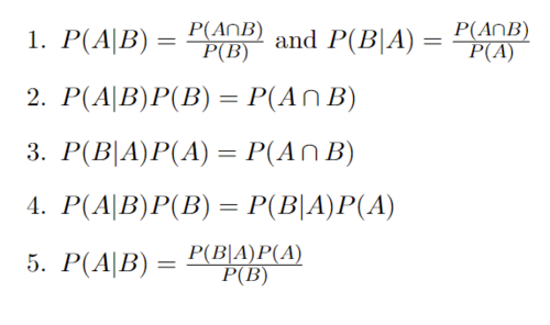
Starting with the definition of Conditional Probability
In Step 1 with the definition of conditional probabilities, it is assumed that P(A) and P(B) are not 0.
In Step 2 we multiply both sides by P(B) and in step 3 we multiply both sides by P(A) and we end up with the same result on the right hand side of each.
In Step 4 we are able to set both left sides equal to each other since they both have the same right hand side.
In Step 5 we divide both sides by P(B) and we arrive at Baye's Theorem.
It is also important to introduce the law of total probability:
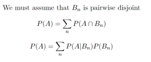
The law of total probability is commonly used in Baye's rule. It is very useful, because it provides a way to calculate probabilities by using conditional probabilities. This is used commonly to compute the denominator when given partitions of the conditional probabilities. A quick example using the law of total probability is:
In this example we are able to solve for the probability of A by just using the probability of A given B, the probability of A given the complement of B, and the probability of B.
Baye's Disease Example:
Say for example that you have tested positive for a disease which affects 0.1% of the population using a test which correctly identifies people who have the disease 99% of the time whilst also only incorrectly identifying people who do not have the disease 1% of the time, meaning that it has a false positive rate of 1%, and a true positive rate of 99%. What is the percent chance that you actually have this disease?
Intuitively, you might say that because the test has a success rate of 99%, then the chance that you actually have this disease is also 99%, but you would actually be incorrect.
In order to find that actual probability that you have this disease, we need to use Bayes Theorem on our data. We want to know the probability of having the disease (D), given that we have tested positive (+), thus we want to find P(D|+). We know the probability of someone having the disease is 0.1%, P(D), we also know the probability of testing positive given that you have the disease is 99% P(+|D), and lastly, we know the probability of testing positive given that you don't have the disease is 1% P(+|D'). By plugging these values into the equation for Baye's Rule, we can find the probability of having the disease given we tested positive:
Applying Baye's Rule:
By applying the law of total probability, we get:
Lastly, by plugging in our values we get:
Our final result states that the probability of you actually having the disease if this test returns positive is only about 9%. This result may seem unintuitive, but will make much more sense when viewed from another perspective.
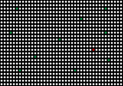
Say, for example, that you have a sample population of 1000 people, then given that the probability that 0.1% of people are affected by this disease, we can say that 1 person in this thousand are likely to have the disease:
If everyone in this sample is given a test for the disease, then it is likely that we will have 10 people who test positive for this disease who do not have the disease (false positives, marked in green), and 1 person who tests positive and does have the disease (true positive, marked in red):
Then the person who actually has the disease and tests positive is only 1 among 11 people in the sample who tested positive.
Thus the probability that your test result is a true positive, is 1/11, or roughly 9%. This, obviously, is not a very conclusive or satisfactory result so what we can do to be absolutely sure is to take another test.
Say that we take the exact same test again and it also returns positive. One thing we can do in Bayesian statistics is update our prior probability with the probability we calculated previously, called the posterior probability. To do this, we now know that the probability that we have the disease is 9%, so we replace the P(D) from our previous equation with P(D) = 0.09:
With this result we can be a lot more certain that we do in fact have this rare disease, but notice that this percentage is still below the 99% success rate of the test. This is simply one of many ways in which people can manipulate and misrepresent statistics. If people were to report that this test is successful 99% of the time, most people would automatically assume that they have the disease if the test returned positive when the chance is actually much lower. There are a lot of ways in which people can trick you with statistics if you aren’t armed with the knowledge to interpret and understand the nuances behind them. This is just one simple example of how seemingly simple statistics at face value, can have surprising and unintuitive meanings.
So how does this apply to the real world? For this we will look at data for COVID 19:
Using data from the CDC, we know that the average weekly number of cases in the United States (that are reported) is 40,102 as of November 18, 2022. Using this value and dividing by the US population from the U.S. census as of November 27, 2022 (333,318,862), we can calculate that the prevalence of COVID-19 in the US is 40,102/333,318,862 = 0.00012031122 = 0.012% = P(D). For this example, we will look at the accuracy of the at home antigen tests. Taking data from a review of studies published by Cochrane, the authors found that in summary, antigen tests used on people who have symptoms showed a false positive rate of 11% P(+|D') and a false negative rate of 1% P(-|D), thus the P(+|D) = 1 - 1% = 99%. Plugging in these values to Bayes rule, we find:
Then if we were to take a second test:
And a third:
TODO: Finish this section, include ethical part and how this data is not accurate.
Sources:
https://www.census.gov/popclock/
https://www.cdc.gov/coronavirus/2019-ncov/covid-data/covidview/index.html


