m |
m |
||
| Line 40: | Line 40: | ||
Then we should look at the speech in frequency domain.<br /> | Then we should look at the speech in frequency domain.<br /> | ||
The analysis tool is Spectrogram, which is based on the codes from [http://engineering.purdue.edu/VISE/ee438L/lab9/pdf/lab9a.pdf Lab 9a-Speech Processing I]. | The analysis tool is Spectrogram, which is based on the codes from [http://engineering.purdue.edu/VISE/ee438L/lab9/pdf/lab9a.pdf Lab 9a-Speech Processing I]. | ||
| − | Spectrogram is a three dimensional diagram,in which the x-axis represents time, y-axis represents frequency and z-axis represents the FFT (fast fourier transform) | + | Spectrogram is a three dimensional diagram,in which the x-axis represents time, y-axis represents frequency and z-axis represents the FFT (fast fourier transform) at each short period of time. It tells us what is the overall distribution of the audio frequency. Based on the diagram, we can determine how to design our bandpass filter. |
| + | {| class="wikitable sortable" | ||
| + | | | ||
| + | | | ||
| + | [[File:Noise 1 Spectrogram.jpg|thumbnail|center|Noise 1 Spectrogram]] | ||
| + | || | ||
| + | [[File:Noise 2 Spectrogram.jpg|thumbnail|center|Noise 2 Spectrogram]] | ||
| + | | | ||
| + | | | ||
| + | [[File:OneSmallStep Spectrogram.jpg|thumbnail|center|OneSmallStep Spectrogram]] | ||
| + | || | ||
| + | [[File:OneGiantLeap Spectrogram.jpg|thumbnail|center|OneGiantLeap Spectrogram]] | ||
| + | |} | ||
| + | <source lang="MATLAB"> | ||
| + | CLEAR; | ||
| + | FileCutting; | ||
| + | delta_t = 40; | ||
| + | overlap = 20; | ||
| + | N = 512; | ||
| + | F1 = figure(1); | ||
| + | autoSpecgm(noise1,f_sampling,delta_t,overlap,N,F1); | ||
| + | title('Noise1') | ||
| + | |||
| + | F2 = figure(2); | ||
| + | autoSpecgm(noise2,f_sampling,delta_t,overlap,N,F2); | ||
| + | title('Noise2') | ||
| + | |||
| + | F3 = figure(3); | ||
| + | autoSpecgm(One_Man,f_sampling,delta_t,overlap,N,F3); | ||
| + | title('One Man') | ||
| + | |||
| + | F4 = figure(4); | ||
| + | autoSpecgm(One_Mankind,f_sampling,delta_t,overlap,N,F4); | ||
| + | title('One Mankind') | ||
| + | |||
| + | function autoSpecgm(signal,fs,delta_t,overlap,N,PIC) | ||
| + | |||
| + | SIGNAL = Specgm(signal,delta_t,overlap,N); | ||
| + | SIGNAL = transpose(SIGNAL); | ||
| + | t = 1:(delta_t-overlap):length(signal); | ||
| + | f = 0:fs/2; | ||
| + | |||
| + | figure(PIC) | ||
| + | subplot(1,2,1) | ||
| + | [row,col] = size(SIGNAL); | ||
| + | imagesc(t,f,abs(SIGNAL(1:row/2,:))) | ||
| + | axis xy | ||
| + | subplot(1,2,2) | ||
| + | mesh(abs(SIGNAL(1:row/2,:))) | ||
| + | end | ||
| + | </source> | ||
| + | From the Spectrogram, we know that the constant noise is concentrated on frequency spectrum about 1-300Hz, whereas the speech | ||
Revision as of 17:43, 23 November 2016
Contents
Introduction
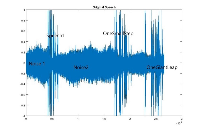
When Neil Armstrong landed on the moon, he said "That's one small step for (a) man; one giant leap for mankind." However,because all the noises (machine vibration,breathing and white noise in radio frequency), people cannot distinguish if he said "a man" or just "man". A lot of experts tried different methods but still could not extract the "a" from the background noise. Hence, the answer is still unknown.
This small project will focus on noise reduction techniques to increase the overall signal to noise ratio (SRN)
Two techniques will be introduced:
- Bandpass Filter
- Noise Gate
Original Speech Analysis
Speech in Time domian
The original speech file can be found from NASA page: July 20, 1969: One Giant Leap For Mankind
Play the audio
While playing the audio, we can hear a constant machine vibration and white noise in the background.
The whole audio can be divided to 5 parts:
We can use MATLAB load the audio file and then divide the audio to different parts.
Here,I divided the audio to five parts.
    [speech,f_sampling] = audioread('Original Speech.wav');
    noise1 = speech(1:3*f_sampling);
    speech1 = speech(round(3.652*f_sampling):round(5.682*f_sampling));
    noise2 = speech(round(5.694*f_sampling):round(15.388*f_sampling));
    One_Man = speech(round(15.337*f_sampling):round(18.584*f_sampling));
    One_Mankind = speech(round(20.633*f_sampling):floor(24.1*f_sampling));
    save noise.mat noise1 noise2
    save Main.mat speech1 One_Man One_Mankind
Speech in Frequency domian
Then we should look at the speech in frequency domain.
The analysis tool is Spectrogram, which is based on the codes from Lab 9a-Speech Processing I.
Spectrogram is a three dimensional diagram,in which the x-axis represents time, y-axis represents frequency and z-axis represents the FFT (fast fourier transform) at each short period of time. It tells us what is the overall distribution of the audio frequency. Based on the diagram, we can determine how to design our bandpass filter.
    CLEAR;
    FileCutting;
    delta_t = 40;
    overlap = 20;
    N = 512;

    F1 = figure(1);
    autoSpecgm(noise1,f_sampling,delta_t,overlap,N,F1);
    title('Noise1')

    F2 = figure(2);
    autoSpecgm(noise2,f_sampling,delta_t,overlap,N,F2);
    title('Noise2')

    F3 = figure(3);
    autoSpecgm(One_Man,f_sampling,delta_t,overlap,N,F3);
    title('One Man')

    F4 = figure(4);
    autoSpecgm(One_Mankind,f_sampling,delta_t,overlap,N,F4);
    title('One Mankind')

    function autoSpecgm(signal,fs,delta_t,overlap,N,PIC)

    SIGNAL = Specgm(signal,delta_t,overlap,N);
    SIGNAL = transpose(SIGNAL);
    t = 1:(delta_t-overlap):length(signal);
    f = 0:fs/2;

    figure(PIC)
    subplot(1,2,1)
    [row,col] = size(SIGNAL);
    imagesc(t,f,abs(SIGNAL(1:row/2,:)))
    axis xy
    subplot(1,2,2)
    mesh(abs(SIGNAL(1:row/2,:)))
    end
From the Spectrogram, we know that the constant noise is concentrated on frequency spectrum about 1-300Hz, whereas the speech


