| (13 intermediate revisions by the same user not shown) | |||
| Line 61: | Line 61: | ||
e) Imagine that the values of <math>(R,G,B)</math> are quantized to 8 bits, and that you view a smooth gradient from black to white on this device. What artifact are you likely to see, and where in the gradient will you see it? | e) Imagine that the values of <math>(R,G,B)</math> are quantized to 8 bits, and that you view a smooth gradient from black to white on this device. What artifact are you likely to see, and where in the gradient will you see it? | ||
| − | :'''Click [[ | + | :'''Click [[CS5_2015_Aug_prob1|here]] to view student [[CS5_2015_Aug_prob1|answers and discussions]]''' |
---- | ---- | ||
===Part 2=== | ===Part 2=== | ||
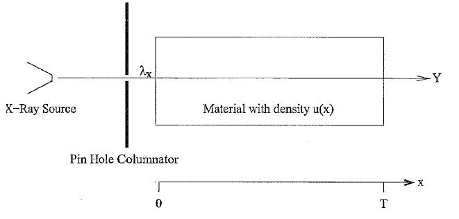
| − | Consider | + | Consider an X-ray imaging system shown in the figure below. <br /> |
| + | [[ Image:Pro2_2015_Aug.PNG ]]<br /> | ||
| + | Photons are emitted from an X-ray source and columnated by a pin hole in a lead shield. The columnated X-rays then pass in a straight line through an object of length T with density u(x) where x is the depth into the object. The number of photons in the beam at depth <math>x</math> is denoted by the random variable <math> Y_x</math> with Poisson density given by | ||
| + | |||
<math> | <math> | ||
| − | + | P\{Y_x = k\} = \frac{e^{-\lambda_x}{\lambda}^{k}_{x}}{k!} . | |
| − | <math> | + | </math> |
| + | |||
| + | Where x is measured in the units of <math>cm</math> and <math>\mu(x)</math> is measured in units of <math>cm^{-1}</math>. | ||
| − | a) Calculate the | + | a) Calculate the mean of <math> Y_x</math>, i.e. <math>E[Y_x]</math>. |
| − | b) Calculate the | + | b) Calculate the variance of <math> Y_x</math>, i.e. <math>E[(Y_x-E[Y_x])^2]</math>. |
| − | c) | + | c) Write a differential equation which describes the behavior of <math>\lambda_x</math> as a function of <math> x</math>. |
| − | d) | + | d) Solve the differential equation to form an expression for <math>\lambda_x</math> in terms of <math>\mu(x)</math> and <math>\lambda_0</math>. |
| − | e) | + | e) Calculate an expression for the integral of the density, <math> \int_{0}^{T} \mu dx </math>, in terms of <math>\lambda_0</math> and <math>\lambda_T</math> |
| − | :'''Click [[ | + | :'''Click [[CS5_2015_Aug_prob2|here]] to view student [[CS5_2015_Aug_prob2|answers and discussions]]''' |
---- | ---- | ||
[[ECE_PhD_Qualifying_Exams|Back to ECE QE page]]: | [[ECE_PhD_Qualifying_Exams|Back to ECE QE page]]: | ||
Latest revision as of 11:53, 7 December 2015
Communication, Networking, Signal and Image Processing (CS)
Question 5: Image Processing
August 2015
Part 1
Consider the emissive display device which is accurately modeled by the equation
$ \left[ {\begin{array}{*{20}{c}} X\\ Y\\ Z \end{array}} \right] = \left[ {\begin{array}{*{20}{c}} a&b&c\\ d&e&f\\ g&h&i \end{array}} \right]\left[ {\begin{array}{*{20}{c}} R\\ G\\ B \end{array}} \right] $
where R, G and B are the red, green, and blue inputs in the range 0 to 255 that are used to modulate physically realizable color primaries.
a) What is the gamma of the device?
b) What are the chromaticity components $ (x_r,y_r), (x_g,y_g) $ and $ (x_b,y_b) $ of the device's three primaries.
c) What are the chromaticity components $ (x_w,y_w) $ of the device's white point.
d) Sketch a chromaticity diagram and plot and label the following on it:
$ \\ 1. (x,y)=(1,0)\\ 2. (x, y) = (0,1)\\ 3. (x, y) = (0,0)\\ 4. (R,G,B) = (255, 0 , 0)\\ 5. (R, G, B) = (0, 255,0)\\ 6. (R,G,B) = (0, 0, 255) $
e) Imagine that the values of $ (R,G,B) $ are quantized to 8 bits, and that you view a smooth gradient from black to white on this device. What artifact are you likely to see, and where in the gradient will you see it?
- Click here to view student answers and discussions
Part 2
Consider an X-ray imaging system shown in the figure below.
Photons are emitted from an X-ray source and columnated by a pin hole in a lead shield. The columnated X-rays then pass in a straight line through an object of length T with density u(x) where x is the depth into the object. The number of photons in the beam at depth $ x $ is denoted by the random variable $ Y_x $ with Poisson density given by
$ P\{Y_x = k\} = \frac{e^{-\lambda_x}{\lambda}^{k}_{x}}{k!} . $
Where x is measured in the units of $ cm $ and $ \mu(x) $ is measured in units of $ cm^{-1} $.
a) Calculate the mean of $ Y_x $, i.e. $ E[Y_x] $.
b) Calculate the variance of $ Y_x $, i.e. $ E[(Y_x-E[Y_x])^2] $.
c) Write a differential equation which describes the behavior of $ \lambda_x $ as a function of $ x $.
d) Solve the differential equation to form an expression for $ \lambda_x $ in terms of $ \mu(x) $ and $ \lambda_0 $.
e) Calculate an expression for the integral of the density, $ \int_{0}^{T} \mu dx $, in terms of $ \lambda_0 $ and $ \lambda_T $
- Click here to view student answers and discussions


