Difference between revisions of "Using Matlab to enhance images" - Rhea

Latest revision as of 23:25, 29 November 2015

*. Introduction

we will learn how to use visual technique in Matlab to Smooth and Sharpen an image .

1. Image Smoothing

The idea behind image smoothing is to use a lowpass filter in order to enhance the look of an image. However, a 3X3 median filter is the filter we are going to use in this operation.

The Median filter matlab code is provided below

_ _ _ _ _ _ _ _

function [ y ] = medianFilter(x)

[m,n]=size(x);

y=x;

for x=2:(m-1)

   for y=2:(n-1)
   
       y(x,y)=median(median(x(x-1:x+1,y-1:y+1)));
   
   end
   

end

_ _ _ _ _ _ _ _

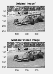
Now we are going to use an example to show image smoothing using the Median filter.

noise1=imread('noise1.tif') noise1_MF=medianFilter(noise1)

figure(1) subplot(2,1,1) image(noise1) colormap(gray(256)) axis('image') title('Original Image"') subplot(2,1,2) image(noise1_MF) colormap(gray(256)) axis('image') title('Median Filtered Image ')

2. Image Sharpening

The idea behind the sharpening technique is to show more details of the image. However, we will use a Gaussian filter to enhance the images.

The Gaussian filter matlab code is provided below

_ _ _ _ _ _ _ _ _ _

function [ d ] = gaussFilter( N, var )

%% where N decides the size of the filter %% var decides the variance of the filter

d=zeros(N)

for n=1:N

   for m=1:N
   
       d(n,m)=exp(-((n-(N+1)/2)^2+(m-(N+1)/2)^2)/(2*var^2))
   
   end
   

end

c=sum(sum(d))

d=d./c

end

_ _ _ _ _ _ _ _ _ _

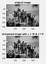
Now we will show an example of using the Gaussian filter.

f=imread('blur.tif') f=double(f) h=gaussFilter(5,1)

figure(1) subplot(2,1,1) image(f) colormap(gray(256)) axis('image') title('original image')

alpha=10 beta=9

    %% alpha and beta are positive constants such that alpha - beta = 1

g2=(alpha.*f)-(beta.*(filter2(h,f)))

subplot(2,1,2) image(g2) colormap(gray(256)) axis('image') title('sharpened image with \alpha = 10 & \beta = 9')

References

Purdue University, "ECE438 - Digital Signal Processing with Applications1ECE438 - Laboratory 10:Image Processing," Purdue University October 6, 2010.