m (Protected "Slecture Relation in frequency Botao Chen" ([Edit=Allow only administrators] (indefinite) [Move=Allow only administrators] (indefinite))) |
|
(No difference)
| |
Revision as of 08:45, 14 March 2015
Frequency domain view of the relationship between a signal and a sampling of that signal
A slecture by ECE student Botao Chen
Partly based on the ECE438 Fall 2014 lecture material of Prof. Mireille Boutin.
Contents
Outline
- Introduction
- Derivation
- Example
- Conclusion
Introduction
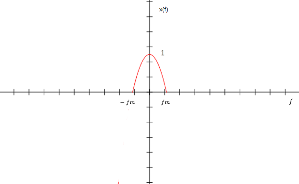
In this slecture I will discuss about the relations between the original signal $ X(f) $ (the CTFT of $ x(t) $ ), sampling continuous time signal $ X_s(f) $ (the CTFT of $ x_s(t) $ ) and sampling discrete time signal $ X_d(\omega) $ (the DTFT of $ x_d[n] $ ) in frequency domain and give a specific example showing the relations.
Derivation
The first thing which need to be clarified is that there two different types of sampling signal: $ x_s(t) $ and $ x_d[n] $. $ x_s(t) $ is created by multiplying a impulse train $ P_T(t) $ with the original signal $ x(t) $ and actually $ x_s(t) $ is $ comb_T(x(t)) $ where T is the sampling period. However the $ x_d[n] $ is $ x(nT) $ where T is the sampling period.
Now we first concentrate on the relationship between $ X(f) $ and $ X_s(f) $.
We know that $ x_s(t) = x(t) \times P_T(t) $, we can derive the relationship between $ x_s(t) $ and $ x(t) $ in the following way:
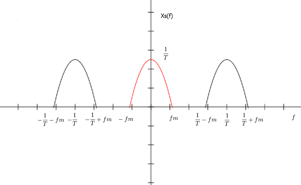
$ \begin{align} F(comb_T(x(t)) &= F(x(t) \times P_T(t))\\ &= X(f)*F(P_T(t))\\ &= X(f)*\frac{1}{T}\sum_{n = -\infty}^\infty \delta(f-\frac{n}{T})\\ &= \frac{1}{T}X(f)*P_\frac{1}{T}(f)\\ &= \frac{1}{T}rep_\frac{1}{T}X(f)\\ \end{align} $
Show this relationship in graph below:
example
Derivation
Then we are going to find the relation between $ X_s(f) $ and $ X_d(\omega) $
We know another way to express CTFT of $ x_s(t) $:
$ \begin{align} X_s(f) &= F(\sum_{n = -\infty}^\infty x(nT)\delta(t-nT))\\ &= \sum_{n = -\infty}^\infty x(nT)F(\delta(t-nT))\\ &= \sum_{n = -\infty}^\infty x(nT)e^{-j2\pi fnT}\\ \end{align} $
compare it with DTFT of $ x_d[n] $:
$ \begin{align} X_d(\omega) &= \sum_{n = -\infty}^\infty x_d[n]e^{-j\omega n}\\ &= \sum_{n = -\infty}^\infty x(nT)e^{-j\omega n}\\ \end{align} $
we can find that:
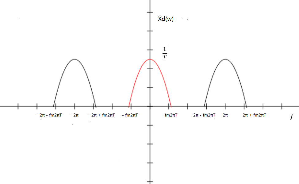
$ \begin{align} X_d(2\pi Tf) &= X_s(f)\\ \end{align} $
if $ f = \frac{1}{T} $
we have that:
$ \begin{align} X_d(2\pi ) &= X_s(\frac{1}{T})\\ \end{align} $
from this equation, we can know the relationship between $ X_s(f) $ and $ X_d(\omega) $ and the relationship is showed in graph as below:
example
conclusion
So the relationship between $ X(f) $ and $ X_s(f) $ is that $ X_s(f) $ is a a rep of $ X(f) $ in frequency domain with period of $ \frac{1}{T} $ and magnitude scaled by $ \frac{1}{T} $. the relationship between $ X(f) $ and $ X_d(\omega) $ is that $ X_d(\omega) $ is also a a rep of $ X(f) $ in frequency domain with period $ 2\pi $ and magnitude is also scaled by $ \frac{1}{T} $, but the frequency is scaled by $ 2\pi T $
Questions and Comments
If you have any questions, comments, etc. please post them on this page.


