| (34 intermediate revisions by 4 users not shown) | |||
| Line 1: | Line 1: | ||
| + | [[Category:slecture]] | ||
| + | [[Category:ECE662Spring2014Boutin]] | ||
| + | [[Category:ECE]] | ||
| + | [[Category:ECE662]] | ||
| + | [[Category:pattern recognition]] | ||
| + | |||
= <center>Introduction to local (nonparametric) density estimation methods</center> = | = <center>Introduction to local (nonparametric) density estimation methods</center> = | ||
| − | <center>A | + | <center>A [http://www.projectrhea.org/learning/slectures.php slecture] by Yu Liu |
| + | |||
| + | Partly based on the [[2014_Spring_ECE_662_Boutin_Statistical_Pattern_recognition_slectures|ECE662 Spring 2014 lecture]] material of [[user:mboutin|Prof. Mireille Boutin]]. | ||
| + | |||
| + | </center> | ||
| + | |||
| + | |||
| + | [[Media:Slecture_introduction_to_local_density_estimation_methods.pdf| click here for PDF version]] | ||
---- | ---- | ||
| − | == '''1. Introduction''' | + | == '''1. Introduction ''' == |
This slecture introduces two local density estimation methods which are Parzen density estimation and k-nearest neighbor density estimation. Local density estimation is also referred to as non-parametric density estimation. To make things clear, let’s first look at parametric density estimation. In parametric density estimation, we can assume that there exists a density function which can be determined by a set of parameters. The set of parameters are estimated from the sample data and are later used in designing the classifier. However, in some practical situations the assumption that there exists a parametric form of the density function does not hold true. For example, it is very hard to fit a multimodal probability distribution with a simple function. In this case, we need to estimate the density function in the nonparametric way, which means that the density function is estimated locally based on a small set of neighboring samples. Because of this locality, local (nonparametric) density estimation is less accurate than parametric density estimation. In the following text the word “local” is preferred over “nonparametric.”<br> | This slecture introduces two local density estimation methods which are Parzen density estimation and k-nearest neighbor density estimation. Local density estimation is also referred to as non-parametric density estimation. To make things clear, let’s first look at parametric density estimation. In parametric density estimation, we can assume that there exists a density function which can be determined by a set of parameters. The set of parameters are estimated from the sample data and are later used in designing the classifier. However, in some practical situations the assumption that there exists a parametric form of the density function does not hold true. For example, it is very hard to fit a multimodal probability distribution with a simple function. In this case, we need to estimate the density function in the nonparametric way, which means that the density function is estimated locally based on a small set of neighboring samples. Because of this locality, local (nonparametric) density estimation is less accurate than parametric density estimation. In the following text the word “local” is preferred over “nonparametric.”<br> | ||
| Line 12: | Line 25: | ||
In local density estimation the density function ''p<sub>n</sub>''(''x'') can be approximated by | In local density estimation the density function ''p<sub>n</sub>''(''x'') can be approximated by | ||
| − | + | <center> [[Image:0f.gif|border]] (1)</center> | |
| − | < | + | |
| − | + | ||
where ''v<sub>n</sub>'' is the volume of a small region ''R'' around point ''x'', ''n'' is the total number of samples ''x''<sub>''i''</sub> (''i'' =1, 2…, ''n'') drawn according to ''p<sub>n</sub>''(''x''), and ''k''<sub>''n''</sub> is the number of ''x''<sub>''i''</sub>’s which fall into region ''R''. The reason why ''p<sub>n</sub>''(''x'') can be calculated in this way is that ''p''<sub>''n''</sub>(''x'') does not vary much within a relatively small region, thus the probability mass of region ''R'' can be approximated by ''p''<sub>''n''</sub>(''x'')''v''<sub>''n''</sub>, which equals ''k''<sub>''n''</sub>/''n''. | where ''v<sub>n</sub>'' is the volume of a small region ''R'' around point ''x'', ''n'' is the total number of samples ''x''<sub>''i''</sub> (''i'' =1, 2…, ''n'') drawn according to ''p<sub>n</sub>''(''x''), and ''k''<sub>''n''</sub> is the number of ''x''<sub>''i''</sub>’s which fall into region ''R''. The reason why ''p<sub>n</sub>''(''x'') can be calculated in this way is that ''p''<sub>''n''</sub>(''x'') does not vary much within a relatively small region, thus the probability mass of region ''R'' can be approximated by ''p''<sub>''n''</sub>(''x'')''v''<sub>''n''</sub>, which equals ''k''<sub>''n''</sub>/''n''. | ||
Some examples of region ''R'' in different dimensions: i) line segment in one-dimension, ii) circle or rectangle in two-dimension, iii) sphere or cube in three-dimension, iv) hyper sphere or hypercube in ''d''-dimension (''d'' > 3). | Some examples of region ''R'' in different dimensions: i) line segment in one-dimension, ii) circle or rectangle in two-dimension, iii) sphere or cube in three-dimension, iv) hyper sphere or hypercube in ''d''-dimension (''d'' > 3). | ||
| − | Three conditions we need to pay attention to when using formula (1) are: | + | Three conditions we need to pay attention to when using formula (1) are: |
| − | + | i)[[Image:1f.gif|border]]. This is because if ''v''<sub>''n''</sub> is fixed, then ''p''<sub>''n''</sub>(''x'') only represents the average probability density as ''n'' grows larger, but what we need is the point probability density, so we should have [[Image:Af.gif|border]] when [[Image:Bf.gif|border]]. | |
| − | + | ii)[[Image:2f.gif|border]]. This is to make sure that we do not get zero probability density. | |
| − | + | iii)[[Image:3f.gif|border]]. This is to make sure that ''p''<sub>''n''</sub>(''x'') does not diverge. | |
| − | + | == '''3. Parzen Density Estimation''' == | |
| − | + | ||
| − | + | ||
| − | + | ||
| − | + | ||
| − | <center> | + | In Parzen density estimation ''v''<sub>''n''</sub> is directly determined by ''n'' while ''k''<sub>''n''</sub> is a random variable which denotes the number of samples that fall into ''v''<sub>''n''</sub>. Assume that the region ''R'' is a ''d''-dimensional hypercube with its edge length ''h''<sub>''n''</sub>, thus <br> |
| + | <center>''v''<sub>''n''</sub> = (''h''<sub>''n''</sub>)''<sup>d</sup>''</center> | ||
| + | <span style="line-height: 1.5em;">The equivalent conditions which meet the aforementioned three conditions are:</span> | ||
| + | <center>[[Image:1f.gif|border]] and [[Image:Ef.gif|border]] </center> | ||
| + | <span style="line-height: 1.5em;">Therefore </span>''v''<sub style="line-height: 1.5em;">''n''</sub><span style="line-height: 1.5em;"> can be chosen as </span>[[Image:Cf.gif|border]]<span style="line-height: 1.5em;"> or </span>[[Image:Df.gif|border]]<span style="line-height: 1.5em;">, where </span>''h''<span style="line-height: 1.5em;"> is an adjustable constant. Now that the relationship between </span>''v''<sub style="line-height: 1.5em;">''n''</sub><span style="line-height: 1.5em;"> and </span>''n''<span style="line-height: 1.5em;"> is defined, the next step is to determine </span>''k''<sub style="line-height: 1.5em;">''n''</sub><span style="line-height: 1.5em;">. To determine </span>''k''<sub style="line-height: 1.5em;">''n''</sub><span style="line-height: 1.5em;">, we define a window function as follows:</span><br> | ||
| + | <center>[[Image:4f.gif|border|center]]</center> | ||
| + | where ''x''<sub>''i''</sub>’s (''i'' = 1, 2, …, ''n'') are the given samples and ''x'' is the point where the density is to be estimated. Thus we have | ||
| + | <center>[[Image:5f.gif|border|center]]</center> <center>[[Image:6f.gif|border|center]]</center> | ||
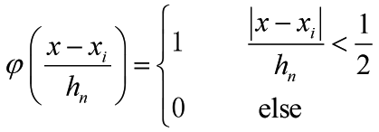
| + | <br>The function [[Image:7f.gif|border]] is called a Parzen window function, which enables us to count the number of sample points in the hypercube with its edge length ''h''<sub>''n''</sub>. According to [2], using hypercube as the window function may lead to discontinuity in the estimation. This is due to the superimposition of sharp pulses centered at the given sample points when h is small. To overcome this shortcoming, we can consider a more general form of window function rather than the hypercube. Note that if the following two conditions are met, the estimated ''p''<sub>''n''</sub>(''x'') is guaranteed to be proper. | ||
| + | <center>[[Image:7f (2).gif|border]] and [[Image:8f.gif|border]]</center> | ||
| + | Therefore a better choice of window function which removes discontinuity can be Gaussian window: | ||
| + | <center>[[Image:9f.gif|border]]</center> | ||
| + | The estimated density is given by | ||
| + | <center> [[Image:10f.gif|border]] <span style="line-height: 1.5em;">(2)</span></center> | ||
| + | Consider a one-dimension case, assume that [[Image:Cf.gif|border]], thus [[Image:Z.gif|border]], where ''h'' is an adjustable constant. Substitute into formula (2) we have | ||
| + | <center>[[Image:11f.gif|border|700x78px]]</center> | ||
| + | <br>We can see that if ''n'' equals one, ''p''<sub>''n''</sub>(''x'') is just the window function. If ''n'' approaches infinity, ''p''<sub>''n''</sub>(''x'') can converge to any complex form. If ''n'' is relatively small, ''p''<sub>''n''</sub>(''x'') is very sensitive to the value of ''h''. In general small ''h'' leads to the noise error while large ''h'' leads to the over-smoothing error, which can be illustrated by the following example. | ||
<br> | <br> | ||
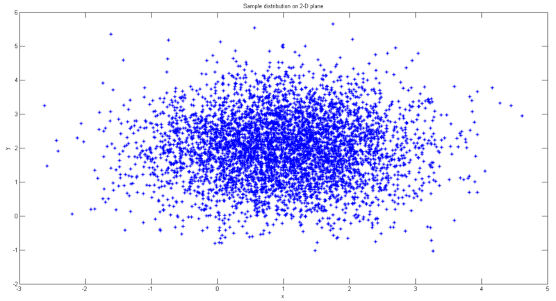
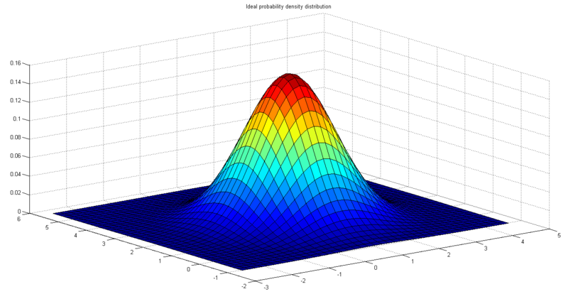
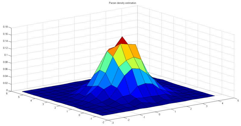
| − | <center>[[Image:3ly.png|border|center|800x600px]]</center> | + | In this experiment samples are 5000 points on 2-D plane with Gaussian distribution. The mean vector is [1 2], and the covariance matrix is [1 0; 0 1]. Choose rectangle Parzen window with [[Image:X.gif|border]], thus [[Image:Y.gif|border]]. Fig. 1 shows the sample distribution. Fig. 2 shows the ideal probability density distribution. Fig. 3 shows the result of Parzen density estimation. |
| − | + | <center>[[Image:1ly.png|border|center|800x600px]]</center> <center>Figure 1. 5000 sample points on 2-D plane with Gaussian distribution</center> <center>[[Image:2ly.png|border|center|800x600px]]</center> <center>Figure 2. The ideal probability density distribution</center> <center>[[Image:3ly.png|border|center|800x600px]]</center> <center>Figure 3. The result of Parzen density estimation</center> | |
| − | <center>Figure 3. The result of Parzen density estimation</center> | + | <br> Next we change the value of ''h''<sub>''n''</sub> and see how it affects the estimation. Fig. 4 shows the result of Parzen density estimation when ''h''<sub>''n''</sub> is twice its initial value. Fig. 5 shows the result of Parzen density estimation when ''h''<sub>''n''</sub> is its initial value divided by two. We can see that the results agree with the aforesaid property of ''h''<sub>''n''</sub>. |
| − | + | <center>[[Image:4ly.png|border|center|800x600px]]</center> <center>Figure 4. The result of Parzen density estimation when ''h''<sub>''n''</sub> is twice its initial value</center> <center>[[Image:5ly.png|border|center|800x600px]]</center> <center>Figure 5. The result of Parzen density estimation when ''h''<sub>''n''</sub> is its initial value divided by two</center> | |
| − | <br> | + | <br> To design a classifier using Parzen window method [3], we estimate the densities for each class and classify the test point by the label corresponding to the maximum posterior. Below lists some advantages and disadvantages of Parzen density estimation: |
| − | + | ||
| − | Next we change the value of ''h''<sub>''n''</sub> and see how it affects the estimation. Fig. 4 shows the result of Parzen density estimation when ''h''<sub>''n''</sub> is twice its initial value. Fig. 5 shows the result of Parzen density estimation when ''h''<sub>''n''</sub> is its initial value divided by two. We can see that the results agree with the aforesaid property of ''h''<sub>''n''</sub>. | + | |
| − | + | ||
| − | <center>[[Image:4ly.png|border|center|800x600px]]</center> | + | |
| − | + | ||
| − | <center>Figure 4. The result of Parzen density estimation when ''h''<sub>''n''</sub> is twice its initial value</center> | + | |
| − | + | ||
| − | + | ||
| − | + | ||
| − | <center>[[Image:5ly.png|border|center|800x600px]]</center> | + | |
| − | + | ||
| − | <center>Figure 5. The result of Parzen density estimation when ''h''<sub>''n''</sub> is its initial value divided by two</center> | + | |
| − | + | ||
| − | <br> | + | |
| − | + | ||
| − | To design a classifier using Parzen window method [3], we estimate the densities for each class and classify the test point by the label corresponding to the maximum posterior. | + | |
| − | + | ||
| − | Below lists some advantages and disadvantages of Parzen density estimation: | + | |
Advantages: i) ''p''<sub>''n''</sub>(''x'') can converge to any complex form when ''n'' approaches infinity; ii) applicable to data with any distribution. | Advantages: i) ''p''<sub>''n''</sub>(''x'') can converge to any complex form when ''n'' approaches infinity; ii) applicable to data with any distribution. | ||
| Line 67: | Line 72: | ||
== '''4. K-Nearest Neighbor Density Estimation''' == | == '''4. K-Nearest Neighbor Density Estimation''' == | ||
| − | In ''k''-nearest neighbor density estimation (use acronym “''k''-NN” in the following text) ''k'' is directly determined by ''n'' while ''v'' is a random variable which denotes the volume that encompasses just ''k'' sample points inside ''v'' and on its boundary. If ''v'' is a sphere, it can be given by< | + | In ''k''-nearest neighbor density estimation (use acronym “''k''-NN” in the following text) ''k'' is directly determined by ''n'' while ''v'' is a random variable which denotes the volume that encompasses just ''k'' sample points inside ''v'' and on its boundary. If ''v'' is a sphere, it can be given by |
| + | <center>[[Image:12f.gif|border]]</center> | ||
| + | <br>where ''h'' is the radius of the sphere with center ''x''. ''h''<sub>''k''</sub> equals ||''x''<sub>''lk''</sub> - ''x''|| where ''x''<sub>''lk''</sub> is the ''k''<sup>th</sup> closest sample point to ''x''. Then the probability density at ''x'' is approximated by | ||
| + | <center> [[Image:13f.gif|border]] <span style="line-height: 1.5em;">(3)</span></center> | ||
| + | where ''k''<sub>1</sub> is number of sample points on the boundary of ''v''<sub>''k''</sub>(''x''). Most of the time formula (3) can be rewritten as | ||
| + | <center>[[Image:14f.gif|border]]</center> | ||
| + | <br>It can be proved that [[Image:15f.gif|border]]. | ||
| − | In Parzen density estimation ''v''<sub>''n''</sub> only depends on ''n'' and is the same for all the test points, while in ''k''-NN ''v<sub><span style="line-height: 1.5em;">n</span></sub>''<u></u><span style="line-height: 1.5em;"> is smaller at high density area and is larger at low density area. This strategy seems more reasonable than the strategy to determine ''v''<sub>''n''</sub> in Parzen density estimation since now ''v''<sub>''n''</sub> is adaptive to the local density.</span> | + | In Parzen density estimation ''v''<sub>''n''</sub> only depends on ''n'' and is the same for all the test points, while in ''k''-NN ''v<sub><span style="line-height: 1.5em;">n</span></sub>''<u></u><span style="line-height: 1.5em;"> is smaller at high density area and is larger at low density area. This strategy seems more reasonable than the strategy to determine ''v''<sub>''n''</sub> in Parzen density estimation since now ''v''<sub>''n''</sub> is adaptive to the local density.</span> In practice, when we want to classify data using ''k''-NN estimation, it turns out that we can get the posterior ''p''(''w''<sub>''i''</sub>|''x'') directly without worrying about ''p''(''x''). If we have ''k'' samples fall into volume ''v'' around point ''x'', and among the ''k'' samples there are ''k''<sub>''i''</sub> samples belonging to class ''w''<sub>''i''</sub>, then we have |
| − | + | <center>[[Image:16f.gif|border]]</center> | |
| − | In practice, when we want to classify data using ''k''-NN estimation, it turns out that we can get the posterior ''p''(''w''<sub>''i''</sub>|''x'') directly without worrying about ''p''(''x''). If we have ''k'' samples fall into volume ''v'' around point ''x'', and among the ''k'' samples there are ''k''<sub>''i''</sub> samples belonging to class ''w''<sub>''i''</sub>, then we have < | + | <br>The posterior ''p''(''w''<sub>''i''</sub>|''x'') is given by |
| − | + | <center> [[Image:17f.gif|border]] <span style="line-height: 1.5em;">(4)</span></center> | |
| − | + | where ''m'' is the number of classes. Formula (4) tells us one simple decision rule: the class of a test point ''x'' is the same as the most frequent one among the nearest ''k'' points of ''x''. Simple and intuitive, isn’t it? Having said that, choosing ''k'' in ''k''-NN is still a nontrivial problem as choosing ''h'' in Parzen density estimation. Small ''k'' leads to noisy decision boundaries while large ''k'' leads to over-smoothed boundaries, which is illustrated by the following example. In this experiment samples are 200 pre-labeled (red or blue) points. The task is to find the classification boundaries under different ''k'' values. Fig. 6-9 show the results. | |
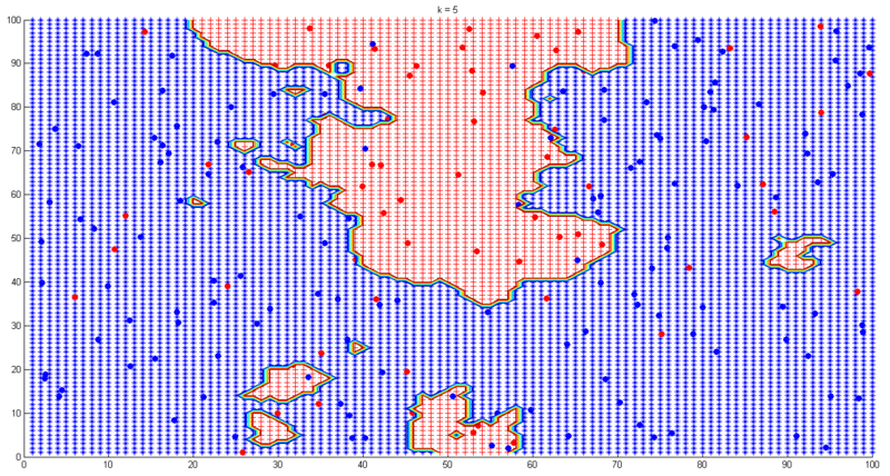
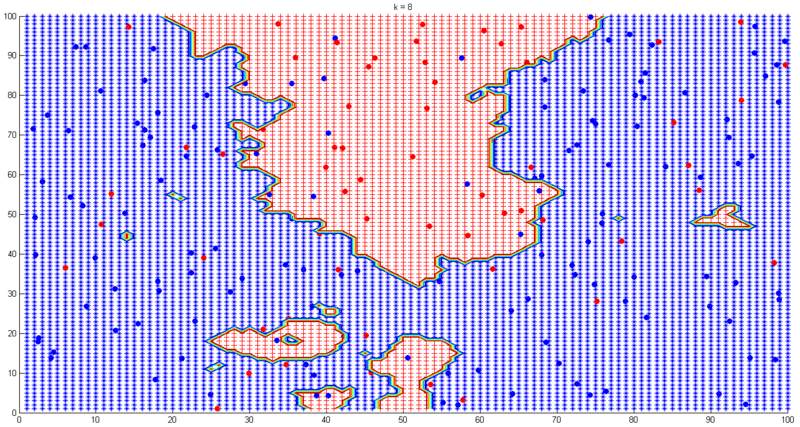
| − | + | <center>[[Image:6ly.png|border|center|800x600px]]</center> <center>Figure 6. ''k''-NN decision boundaries experiment (''k''=2)</center> <center></center> <center>[[Image:7ly.png|border|center|800x600px]]</center> <center>Figure 7. ''k''-NN decision boundaries experiment (''k''=3)</center> <center></center> <center>[[Image:8ly.png|border|center|800x600px]]</center> <center>Figure 8. ''k''-NN decision boundaries experiment (''k''=5)</center> <center></center> <center>[[Image:9ly.png|border|center|800x600px]]</center> <center>Figure 9. ''k''-NN decision boundaries experiment (''k''=8)</center> | |
| − | In this experiment samples are | + | <br> In practice we can use cross-validation to choose the “best” ''k''. Below lists some advantages and disadvantages of ''k''-NN: |
| − | + | ||
| − | <center>[[Image:6ly.png|border|center|800x600px]]</center> | + | |
| − | <center>Figure 6. ''k''-NN decision boundaries experiment (''k''=2)</center> | + | |
| − | + | ||
| − | < | + | |
| − | + | ||
| − | <center>[[Image:7ly.png|border|center|800x600px]]</center> | + | |
| − | <center>Figure 7. ''k''-NN decision boundaries experiment (''k''=3)</center> | + | |
| − | + | ||
| − | < | + | |
| − | + | ||
| − | <center>[[Image:8ly.png|border|center|800x600px]]</center> | + | |
| − | <center>Figure 8. ''k''-NN decision boundaries experiment (''k''=5)</center> | + | |
| − | + | ||
| − | < | + | |
| − | + | ||
| − | <center>[[Image:9ly.png|border|center|800x600px]]</center> | + | |
| − | <center>Figure 9. ''k''-NN decision boundaries experiment (''k''=8)</center> | + | |
| − | + | ||
| − | <br> | + | |
| − | + | ||
| − | In practice we can use cross-validation to choose the “best” ''k''. Below lists some advantages and disadvantages of ''k''-NN: | + | |
Advantages: i) decision performance is good if ''n'' is large enough; ii) applicable to data with any distribution; iii) simple and intuitive. | Advantages: i) decision performance is good if ''n'' is large enough; ii) applicable to data with any distribution; iii) simple and intuitive. | ||
| Line 105: | Line 94: | ||
== '''5. Reference''' == | == '''5. Reference''' == | ||
| − | [1] Mireille Boutin, “ECE662: Statistical Pattern Recognition and Decision Making Processes,” Purdue University, Spring 2014<br>[2] http://www.cse.buffalo.edu/~jcorso/t/CSE555/files/annote_28feb_nonprm.pdf<br>[3] http://www.csd.uwo.ca/~olga/Courses/CS434a_541a/Lecture6.pdf<br><br><br> | + | [1] Mireille Boutin, “ECE662: Statistical Pattern Recognition and Decision Making Processes,” Purdue University, Spring 2014<br>[2] http://www.cse.buffalo.edu/~jcorso/t/CSE555/files/annote_28feb_nonprm.pdf<br>[3] http://www.csd.uwo.ca/~olga/Courses/CS434a_541a/Lecture6.pdf<br><br><br> |
| + | |||
| + | ---- | ||
| + | ==[[slecture_Introduction_to_local_density_estimation_methods_review|Questions and comments]]== | ||
| + | If you have any questions, comments, etc. please post them on [[slecture_Introduction_to_local_density_estimation_methods_review|this page]]. | ||
Latest revision as of 10:52, 22 January 2015
Contents
Introduction to local (nonparametric) density estimation methods
Partly based on the ECE662 Spring 2014 lecture material of Prof. Mireille Boutin.
1. Introduction
This slecture introduces two local density estimation methods which are Parzen density estimation and k-nearest neighbor density estimation. Local density estimation is also referred to as non-parametric density estimation. To make things clear, let’s first look at parametric density estimation. In parametric density estimation, we can assume that there exists a density function which can be determined by a set of parameters. The set of parameters are estimated from the sample data and are later used in designing the classifier. However, in some practical situations the assumption that there exists a parametric form of the density function does not hold true. For example, it is very hard to fit a multimodal probability distribution with a simple function. In this case, we need to estimate the density function in the nonparametric way, which means that the density function is estimated locally based on a small set of neighboring samples. Because of this locality, local (nonparametric) density estimation is less accurate than parametric density estimation. In the following text the word “local” is preferred over “nonparametric.”
It is noteworthy that it is very difficult to obtain an accurate local density estimation, especially when the dimension of the feature space is high. So why do we bother using local density estimation? This is because our goal is not to get an accurate estimation, but rather to use the estimation to design a well performed classifier. The inaccuracy of local density estimation does not necessarily lead to a poor decision rule.
2. General Principle
In local density estimation the density function pn(x) can be approximated by
 (1)
(1)where vn is the volume of a small region R around point x, n is the total number of samples xi (i =1, 2…, n) drawn according to pn(x), and kn is the number of xi’s which fall into region R. The reason why pn(x) can be calculated in this way is that pn(x) does not vary much within a relatively small region, thus the probability mass of region R can be approximated by pn(x)vn, which equals kn/n.
Some examples of region R in different dimensions: i) line segment in one-dimension, ii) circle or rectangle in two-dimension, iii) sphere or cube in three-dimension, iv) hyper sphere or hypercube in d-dimension (d > 3).
Three conditions we need to pay attention to when using formula (1) are:
i)![]() . This is because if vn is fixed, then pn(x) only represents the average probability density as n grows larger, but what we need is the point probability density, so we should have
. This is because if vn is fixed, then pn(x) only represents the average probability density as n grows larger, but what we need is the point probability density, so we should have ![]() when
when ![]() .
.
ii)![]() . This is to make sure that we do not get zero probability density.
. This is to make sure that we do not get zero probability density.
iii)![]() . This is to make sure that pn(x) does not diverge.
. This is to make sure that pn(x) does not diverge.
3. Parzen Density Estimation
In Parzen density estimation vn is directly determined by n while kn is a random variable which denotes the number of samples that fall into vn. Assume that the region R is a d-dimensional hypercube with its edge length hn, thus
The equivalent conditions which meet the aforementioned three conditions are:
Therefore vn can be chosen as ![]() or
or ![]() , where h is an adjustable constant. Now that the relationship between vn and n is defined, the next step is to determine kn. To determine kn, we define a window function as follows:
, where h is an adjustable constant. Now that the relationship between vn and n is defined, the next step is to determine kn. To determine kn, we define a window function as follows:
where xi’s (i = 1, 2, …, n) are the given samples and x is the point where the density is to be estimated. Thus we have
The function ![]() is called a Parzen window function, which enables us to count the number of sample points in the hypercube with its edge length hn. According to [2], using hypercube as the window function may lead to discontinuity in the estimation. This is due to the superimposition of sharp pulses centered at the given sample points when h is small. To overcome this shortcoming, we can consider a more general form of window function rather than the hypercube. Note that if the following two conditions are met, the estimated pn(x) is guaranteed to be proper.
is called a Parzen window function, which enables us to count the number of sample points in the hypercube with its edge length hn. According to [2], using hypercube as the window function may lead to discontinuity in the estimation. This is due to the superimposition of sharp pulses centered at the given sample points when h is small. To overcome this shortcoming, we can consider a more general form of window function rather than the hypercube. Note that if the following two conditions are met, the estimated pn(x) is guaranteed to be proper.

Therefore a better choice of window function which removes discontinuity can be Gaussian window:

The estimated density is given by
 (2)
(2)Consider a one-dimension case, assume that ![]() , thus
, thus ![]() , where h is an adjustable constant. Substitute into formula (2) we have
, where h is an adjustable constant. Substitute into formula (2) we have

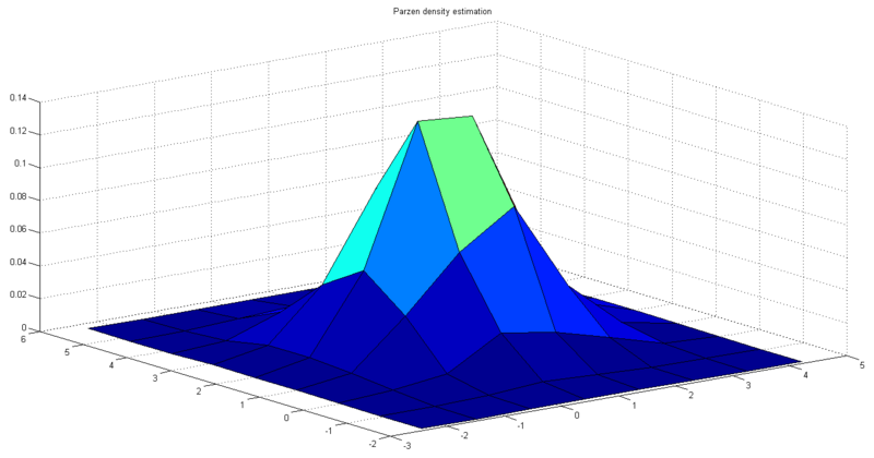
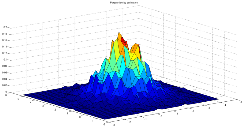
We can see that if n equals one, pn(x) is just the window function. If n approaches infinity, pn(x) can converge to any complex form. If n is relatively small, pn(x) is very sensitive to the value of h. In general small h leads to the noise error while large h leads to the over-smoothing error, which can be illustrated by the following example.
In this experiment samples are 5000 points on 2-D plane with Gaussian distribution. The mean vector is [1 2], and the covariance matrix is [1 0; 0 1]. Choose rectangle Parzen window with ![]() , thus
, thus ![]() . Fig. 1 shows the sample distribution. Fig. 2 shows the ideal probability density distribution. Fig. 3 shows the result of Parzen density estimation.
. Fig. 1 shows the sample distribution. Fig. 2 shows the ideal probability density distribution. Fig. 3 shows the result of Parzen density estimation.
Next we change the value of hn and see how it affects the estimation. Fig. 4 shows the result of Parzen density estimation when hn is twice its initial value. Fig. 5 shows the result of Parzen density estimation when hn is its initial value divided by two. We can see that the results agree with the aforesaid property of hn.
To design a classifier using Parzen window method [3], we estimate the densities for each class and classify the test point by the label corresponding to the maximum posterior. Below lists some advantages and disadvantages of Parzen density estimation:
Advantages: i) pn(x) can converge to any complex form when n approaches infinity; ii) applicable to data with any distribution.
Disadvantages: i) need a large number of samples to obtain an accurate estimation; ii) computationally expensive, not suitable for feature space with very high dimensions; iii) the adjustable constant h has a relatively heavy influence on the decision boundaries when n is small, and is not easy to choose in practice.
4. K-Nearest Neighbor Density Estimation
In k-nearest neighbor density estimation (use acronym “k-NN” in the following text) k is directly determined by n while v is a random variable which denotes the volume that encompasses just k sample points inside v and on its boundary. If v is a sphere, it can be given by
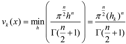
where h is the radius of the sphere with center x. hk equals ||xlk - x|| where xlk is the kth closest sample point to x. Then the probability density at x is approximated by
 (3)
(3)where k1 is number of sample points on the boundary of vk(x). Most of the time formula (3) can be rewritten as

In Parzen density estimation vn only depends on n and is the same for all the test points, while in k-NN vn is smaller at high density area and is larger at low density area. This strategy seems more reasonable than the strategy to determine vn in Parzen density estimation since now vn is adaptive to the local density. In practice, when we want to classify data using k-NN estimation, it turns out that we can get the posterior p(wi|x) directly without worrying about p(x). If we have k samples fall into volume v around point x, and among the k samples there are ki samples belonging to class wi, then we have

The posterior p(wi|x) is given by
 (4)
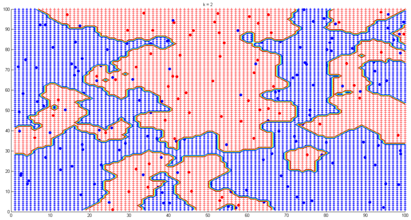
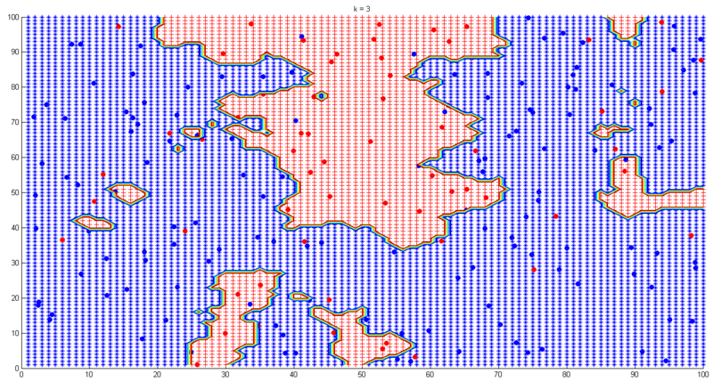
(4)where m is the number of classes. Formula (4) tells us one simple decision rule: the class of a test point x is the same as the most frequent one among the nearest k points of x. Simple and intuitive, isn’t it? Having said that, choosing k in k-NN is still a nontrivial problem as choosing h in Parzen density estimation. Small k leads to noisy decision boundaries while large k leads to over-smoothed boundaries, which is illustrated by the following example. In this experiment samples are 200 pre-labeled (red or blue) points. The task is to find the classification boundaries under different k values. Fig. 6-9 show the results.
In practice we can use cross-validation to choose the “best” k. Below lists some advantages and disadvantages of k-NN:
Advantages: i) decision performance is good if n is large enough; ii) applicable to data with any distribution; iii) simple and intuitive.
Disadvantages: i) need a large number of samples to obtain an accurate estimation, which is inevitable in local density estimation; ii) computationally expensive, low efficiency for feature space with very high dimensions; iii) choosing the “best” k is nontrivial.
5. Reference
[1] Mireille Boutin, “ECE662: Statistical Pattern Recognition and Decision Making Processes,” Purdue University, Spring 2014
[2] http://www.cse.buffalo.edu/~jcorso/t/CSE555/files/annote_28feb_nonprm.pdf
[3] http://www.csd.uwo.ca/~olga/Courses/CS434a_541a/Lecture6.pdf
Questions and comments
If you have any questions, comments, etc. please post them on this page.

