| Line 12: | Line 12: | ||
== <font size="3"></font><font size="3"></font>Outline == | == <font size="3"></font><font size="3"></font>Outline == | ||
| + | |||
| + | <font size="3"></font> | ||
<font size="3"> | <font size="3"> | ||
| Line 33: | Line 35: | ||
Downsampling is an operation which involves throwing away samples from discrete-time signal. Let ''x[n]'' be a digital-time signal shown below: <br> | Downsampling is an operation which involves throwing away samples from discrete-time signal. Let ''x[n]'' be a digital-time signal shown below: <br> | ||
| − | + | [[Image:Xofn.jpg]]<br> | |
then y[n] will be produced by downsampling ''x [n]'' by factor ''D'' = 3. So, ''y [n] = x[Dn]''. | then y[n] will be produced by downsampling ''x [n]'' by factor ''D'' = 3. So, ''y [n] = x[Dn]''. | ||
| − | + | [[Image:Yofn.jpg]]<br> | |
As seen in above graph, ''y [n]'' is obtained by throwing away some samples from x [n]. So, ''y [n]'' is a downsampled signal from | As seen in above graph, ''y [n]'' is obtained by throwing away some samples from x [n]. So, ''y [n]'' is a downsampled signal from | ||
| Line 109: | Line 111: | ||
== Conclusion == | == Conclusion == | ||
</font> | </font> | ||
| + | |||
| + | <font size="3"></font> | ||
<font size="3"></font> | <font size="3"></font> | ||
Revision as of 06:28, 10 October 2014
Downsampling
A slecture by ECE student Yerkebulan Yeshmukhanbetov
Partly based on the ECE438 Fall 2014 lecture material of Prof. Mireille Boutin.
Contents
Outline
- Introduction
- Definition of Downsampling
- Derivation of DTFT of downsampled signal
- Example
- Conclusion
- References
Introduction
This slecture provides definition of downsampling, derives DTFT downsampled signal and demonstrates it in a frequency domain. Also, it explains process of decimation and why it needs a low-pass filter.
Definition of Downsampling
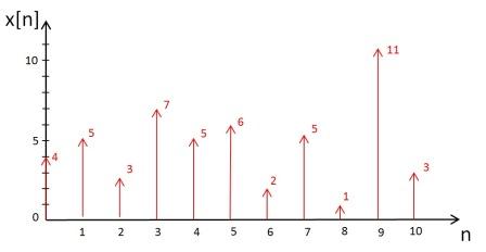
Downsampling is an operation which involves throwing away samples from discrete-time signal. Let x[n] be a digital-time signal shown below:
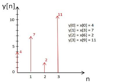
then y[n] will be produced by downsampling x [n] by factor D = 3. So, y [n] = x[Dn].
As seen in above graph, y [n] is obtained by throwing away some samples from x [n]. So, y [n] is a downsampled signal from
x [n].
Derivation of DTFT of downsampled signal
Let x (t) be a continuous time signal. Then x1 [n] = x (T1n) and x2 [n] = x (T2n). And ratio of sampling periods would be
D = T2/T1, which is an integer greater than 1. From these equations we obtain realtionship between x1 [n] and x2 [n].
$ \begin{align} x_2 [n] = x(T_2 n) = x(DT_1 n) = x_1 [nD] \end{align} $
Below we derive Discrete-Time Fourier Transform of x2 [n] in terms of DTFT of x1 [n].
$ \begin{align} &\mathcal{X}_2(\omega)= \mathcal{F}(x_2 [n]) = \mathcal{F}(x_1 [Dn])\\ &= \sum_{n = -\infty}^\infty x_1[Dn] e^{-j \omega n} = \sum_{m = -\infty}^\infty x_1[m] e^{-j \omega {\frac{m}{D}}}\\ &= \sum_{n = -\infty}^\infty s_D[m]* x_1 [m] e^{-j \omega {\frac{m}{D}}}\\ \end{align} $
where
$ s_D [m]=\left\{ \begin{array}{ll} 1,& \text{ if } n \text{ is a multiple of } 4,\\ 0, & \text{ else}. \end{array}\right. = {\frac{1}{D}} \sum_{k = -\infty}^{D-1} e^{jk {\frac{2 \pi}{D} m}} $
$ \begin{align} &\mathcal{X}_2(\omega)= \sum_{m = -\infty}^\infty {\frac{1}{D}} \sum_{k = -\infty}^{D-1} e^{jk {\frac{2 \pi}{D} m}} x_1[m] e^{-j \omega {\frac{m}{D}}}\\ &= {\frac{1}{D}} \sum_{k = -\infty}^{D-1} \sum_{m = -\infty}^\infty x_1[m] e^{-jm ({\frac{\omega - 2 \pi k}{D}})} = \\ &= {\frac{1}{D}} \sum_{k = -\infty}^{D-1} \mathcal{X}_1 ({\frac{\omega - 2 \pi k}{D}}) \\ \end{align} $
Example
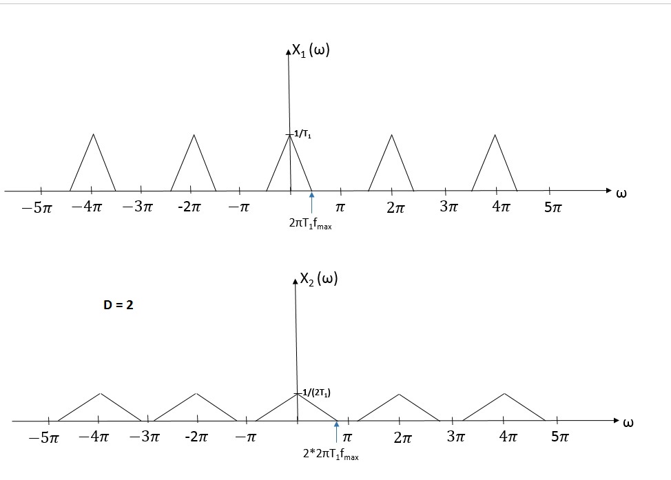
Let's take a look at an original signal X1 (w) and X2 (w) which is obtained after downsampling X1(w) by factor D = 2 in a frequency domain.
Downsampler is a part of a decimator which also has a low-pass filter to prevent aliasing. LPF reduces signal components which has frequencies higher than cutoff frequency, which can be found from graphs shown above.
$ \begin{align} & D 2 \pi T_1 f_{max} < \pi\\ & {\frac{T_2}{T_1}} 2\pi T_1 f_{max} < \pi \\ & 2\pi T_2f_{max} < \pi \\ &f_{max} < {\frac{1}{2T_2}} \end{align} $
Conclusion
To summarize, when signal is downsampled its .
References
[1] John G. Proakis, Dimitris G. Manolakis, "Digital Signal Processing with Principles, Algorithms, and Applications" 4th Edition,2006
Questions and comments
If you have any questions, comments, etc. please post them on this page.


