| Line 4: | Line 4: | ||
<center>[[Image:fig2_color_mh.png|750px|thumb|left|Fig 2: Scatter plots and Contours. All contours are at Mahalanobis distance 1. (a) Original white density of '''W''', (b) scaled density of '''Y''', (c) colored density of '''X'''.]]</center> | <center>[[Image:fig2_color_mh.png|750px|thumb|left|Fig 2: Scatter plots and Contours. All contours are at Mahalanobis distance 1. (a) Original white density of '''W''', (b) scaled density of '''Y''', (c) colored density of '''X'''.]]</center> | ||
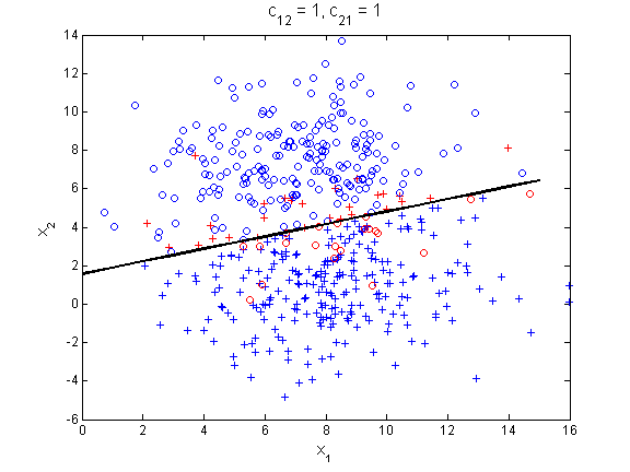
| − | <center>[[Image:C21_5.png|600px|thumb|left|Fig | + | <center>[[Image:C12_1.png|600px|thumb|left|Fig 1(a): <math> c_{12} = 1 , c_{21} = 1 |
| + | </math>Summary diagram of whitening and coloring process.]]</center> | ||
| + | |||
| + | <center>[[Image:C12_5.png|600px|thumb|left|Fig 1(b): <math> c_{12} = 5 , c_{21} = 1 </math>Summary diagram of whitening and coloring process.]]</center> | ||
| + | |||
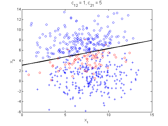
| + | <center>[[Image:C21_5.png|600px|thumb|left|Fig 1(c): <math> c_{12} = 1 , c_{21} = 5 </math>Summary diagram of whitening and coloring process.]]</center> | ||
---- | ---- | ||
Revision as of 16:26, 5 April 2014
test test
References
[2]. Mireille Boutin, "ECE662: Statistical Pattern Recognition and Decision Making Processes," Purdue University, Spring 2014.


