| Line 7: | Line 7: | ||
<math> | <math> | ||
| − | X_{t+1} = | + | X_{t+1} = \mathrm{M}X_t\mathrm{e}^{-j|\mathrm{R}|},\; \mathrm{where} \;\; \mathrm{M} \sim \mathcal{N}(1,.01),\; \mathrm{R} \sim \mathcal{N}(0, .01) |
</math> | </math> | ||
| Line 30: | Line 30: | ||
% generate next states (probabilistic modifications on current state) | % generate next states (probabilistic modifications on current state) | ||
for j=2:length(walk), | for j=2:length(walk), | ||
| − | walk(j) = walk(j-1)*normrnd(1,std_noise_mag)*( | + | walk(j) = walk(j-1)*normrnd(1,std_noise_mag)*(exp(-i*abs(normrnd(0,std_rot)))); |
end; | end; | ||
plot(walk); grid on; hold on; | plot(walk); grid on; hold on; | ||
Revision as of 15:18, 3 March 2013
Markov Processes
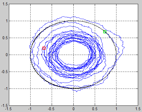
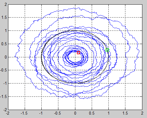
I attempted to model a robot circulating about the origin with small noise in each step. You can directly plug in the Matlab code below. It generated the following images, showing the putative robot spiraling 'inward' or 'outward'. Normally distributed random variables are used to modify the magnitude (M) of the complex vector and rotate the vector in a clockwise direction with a rotation (R) r.v. during each state transition.
The (first-order, stationary, discrete time, continuous state-space) Markov process representing this simple 'walk' is as follows:
$ X_{t+1} = \mathrm{M}X_t\mathrm{e}^{-j|\mathrm{R}|},\; \mathrm{where} \;\; \mathrm{M} \sim \mathcal{N}(1,.01),\; \mathrm{R} \sim \mathcal{N}(0, .01) $
Question: Is the noise early in the walk process has a greater effect on the final position of the robot than noise later in the walk process, suggesting a butterfly effect? It seems that the second image appears to suggest otherwise, since the robot spirals out early but later spirals inward ending at the red square.
% set params
num_steps = 10000;
std_rot = .01;
std_noise_mag = .01;

% generate random initial state with complex magnitude 1
walk = zeros(1,num_steps);
walk(1) = exp(i*rand);
% generate next states (probabilistic modifications on current state)
for j=2:length(walk),
  walk(j) = walk(j-1)*normrnd(1,std_noise_mag)*(exp(-i*abs(normrnd(0,std_rot))));
end;
plot(walk); grid on; hold on;

% plot starting (green) and end (red) markers
plot(walk(1), 'gs','LineWidth', 2);
plot(walk(length(walk)), 'rs','LineWidth', 2);

% generate black circle to compare with "robot" circulation
circ = zeros(1,1000);
circ(1) = i;
for j=2:length(circ),
  circ(j) = circ(j-1)*i^(2*pi/length(circ));
end;
plot(circ,':k','LineWidth', 2); hold off;


