| Line 20: | Line 20: | ||
</math> | </math> | ||
| − | Our input function '''x''' is a constant 1. You can think of this as a Kronecker delta function occurring at every discrete time step, and therefore causing the impulse reponse to 'go off' at every time step ( | + | Our input function '''x''' is a constant 1. You can think of this as a Kronecker delta function occurring at every discrete time step, and therefore causing the impulse reponse to 'go off' at every time step. (However, this does not complete translate to the CT case as we will see.) What we term the 'convolution' is just the summation of all these time-shifted impulse reponses at the time we want to find the convolution for (ie time n for y[n]). To more tangibly express 'summation of all these time-shifted impulse reponses', we can consider an impulse that was generated at time n=0. We know that output from that singular impulse response should be <math style='inline'>(1)(e^{0}) = 1</math> at n=0, <math style='inline'>(1)(e^{-1}) = e^{-1}</math> at n=1, <math style='inline'>(1)(e^{-2}) = e^{-2}</math> at n=2, and so on. But because we have a constant input signal that effectively serves as a delta function at each time step, another impulse would be generated at n=1, yielding <math style='inline'>(1)(0) = 0</math> at n=0, <math style='inline'>(1)(e^{0}) = 1</math> at n=1, <math style='inline'>(1)(e^{-1}) = e^{-1}</math> at n=2, and so on. Look at what's occurring at n=1 here: the convolution will yield <math style='inline'>1 + e^{-1}</math> for the two impulse responses started at time n=0 and n=1. But if we carry this back to earlier impulse responses, we see that we get the geometric series: |
<math> \sum_{k=0}^{\infty} \mathrm{e}^{-k} \,=\, 1 + \frac{1}{e} + \frac{1}{e^2} + \frac{1}{e^3} + ... \,=\, \frac{1}{1-\frac{1}{e}} \,\approx\, 1.582</math> | <math> \sum_{k=0}^{\infty} \mathrm{e}^{-k} \,=\, 1 + \frac{1}{e} + \frac{1}{e^2} + \frac{1}{e^3} + ... \,=\, \frac{1}{1-\frac{1}{e}} \,\approx\, 1.582</math> | ||
| − | Without even resorting to the convolution formula given to us in class, we intuitively grasped what the convolution should be for any time n (doesn't matter what n we choose since input has always been and will always be the same) | + | Without even resorting to the convolution formula given to us in class, we intuitively grasped what the convolution should be for any time n, and calculated the output y[n] for all n. (It doesn't matter what n we choose since input has always been and will always be the same.) Again to clarify, the impulse response calculated here was just the (additive) superposition of time-shifted impulse functions. And because our input is 1 for all n, each of those superimposed impulse responses is scaled with constant coefficient of 1, simplifying our computation to a geometric series. |
[[image:Ec1_2.PNG| 320x320px]][[image:Ec1_1.PNG| 320x320px]][[image:Ec1_3.PNG| 320x320px]] | [[image:Ec1_2.PNG| 320x320px]][[image:Ec1_1.PNG| 320x320px]][[image:Ec1_3.PNG| 320x320px]] | ||
| Line 32: | Line 32: | ||
Now that we've figured out the discrete time case, let's consider the continuous case of these same input and impulse response functions, now defined for all t instead of at discrete intervals n. Using the same intuition as before, in which we consider additive superposition of identically scaled but time-shifted impulse response, we see that instead of having a ''countably infinite'' number of values to add (eg <math style='inline'>1, e^{-1}, e^{-2}, ...</math>) that '''last for a DT step of 1''' (crucial to note this), we now have an ''uncountably infinite'' number of values to add (starting with 1, <math style='inline'>1^-, ...</math>). However, these uncountably infinite values along the continuous input and impulse reponses are ''not'' held for a time step of one each. Instead, the only are held for an infinitesimal amount of time, and thus we must resort to the more traditional integral to calculate the convolution in this CT case instead of using the Riemann integral approach like we implicitly did in the DT case. | Now that we've figured out the discrete time case, let's consider the continuous case of these same input and impulse response functions, now defined for all t instead of at discrete intervals n. Using the same intuition as before, in which we consider additive superposition of identically scaled but time-shifted impulse response, we see that instead of having a ''countably infinite'' number of values to add (eg <math style='inline'>1, e^{-1}, e^{-2}, ...</math>) that '''last for a DT step of 1''' (crucial to note this), we now have an ''uncountably infinite'' number of values to add (starting with 1, <math style='inline'>1^-, ...</math>). However, these uncountably infinite values along the continuous input and impulse reponses are ''not'' held for a time step of one each. Instead, the only are held for an infinitesimal amount of time, and thus we must resort to the more traditional integral to calculate the convolution in this CT case instead of using the Riemann integral approach like we implicitly did in the DT case. | ||
| − | Looking below at the mathematical breakdown of this convolution in CT, we see that the result happens to equal exactly 1, which is significantly less than our result in the DT case. Intuitively, this is because the 'large' early values (eg <math style='inline'>1, e^{-1} = .368, e^{-2} = .135</math>) of the quickly decaying impulse response are held for a time step of 1 each in the DT case, while those values are only held for an infinitesimal time in the CT case. This leads to an interesting conclusion: '''a discrete-time convolution may vary significantly from its continuous-time counterpart'''. | + | Looking below at the mathematical breakdown of this convolution in CT, we see that the result happens to equal exactly 1, which is significantly less than our result in the DT case. Intuitively, this is because the 'large' early values (eg <math style='inline'>e^{0} = 1, e^{-1} = .368, e^{-2} = .135</math>) of the quickly decaying impulse response are held for a time step of 1 each in the DT case, while those values are only held for an infinitesimal time in the CT case. This leads to an interesting conclusion: '''a discrete-time convolution may vary significantly from its continuous-time counterpart'''. |
---- | ---- | ||
Revision as of 09:19, 11 February 2013
Convolution
Convolution is often presented in a manner that emphasizes efficient calculation over comprehension of the convolution itself. To calculate in a pointwise fashion, we're told: "flip one of the input signals, and perform shift+multiply+add operations until the signals no longer overlap." This is numerically valid, but you could in fact calculate the convolution without flipping either signals. We'll perform the latter here for illustration. Consider the convolution of the following constant input and causal impulse reponse:
$ y[n] \,=\, x[n] \ast h[n] $
$ x[n] \,=\, 1 \;\;\;\;\; \forall \, n $
$ h[n] = \left\{ \begin{array}{lr} \mathrm{e}^{-n} & : n \geq 0\\ 0 & : n < 0 \end{array} \right. $
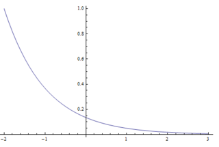
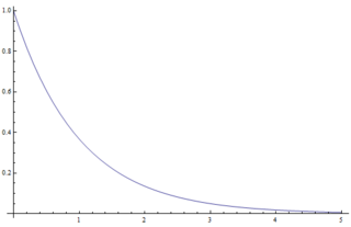
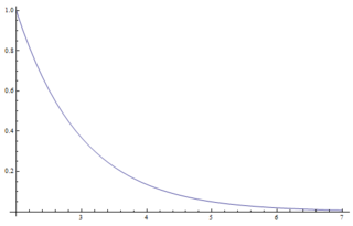
Our input function x is a constant 1. You can think of this as a Kronecker delta function occurring at every discrete time step, and therefore causing the impulse reponse to 'go off' at every time step. (However, this does not complete translate to the CT case as we will see.) What we term the 'convolution' is just the summation of all these time-shifted impulse reponses at the time we want to find the convolution for (ie time n for y[n]). To more tangibly express 'summation of all these time-shifted impulse reponses', we can consider an impulse that was generated at time n=0. We know that output from that singular impulse response should be $ (1)(e^{0}) = 1 $ at n=0, $ (1)(e^{-1}) = e^{-1} $ at n=1, $ (1)(e^{-2}) = e^{-2} $ at n=2, and so on. But because we have a constant input signal that effectively serves as a delta function at each time step, another impulse would be generated at n=1, yielding $ (1)(0) = 0 $ at n=0, $ (1)(e^{0}) = 1 $ at n=1, $ (1)(e^{-1}) = e^{-1} $ at n=2, and so on. Look at what's occurring at n=1 here: the convolution will yield $ 1 + e^{-1} $ for the two impulse responses started at time n=0 and n=1. But if we carry this back to earlier impulse responses, we see that we get the geometric series:
$ \sum_{k=0}^{\infty} \mathrm{e}^{-k} \,=\, 1 + \frac{1}{e} + \frac{1}{e^2} + \frac{1}{e^3} + ... \,=\, \frac{1}{1-\frac{1}{e}} \,\approx\, 1.582 $
Without even resorting to the convolution formula given to us in class, we intuitively grasped what the convolution should be for any time n, and calculated the output y[n] for all n. (It doesn't matter what n we choose since input has always been and will always be the same.) Again to clarify, the impulse response calculated here was just the (additive) superposition of time-shifted impulse functions. And because our input is 1 for all n, each of those superimposed impulse responses is scaled with constant coefficient of 1, simplifying our computation to a geometric series.
Now that we've figured out the discrete time case, let's consider the continuous case of these same input and impulse response functions, now defined for all t instead of at discrete intervals n. Using the same intuition as before, in which we consider additive superposition of identically scaled but time-shifted impulse response, we see that instead of having a countably infinite number of values to add (eg $ 1, e^{-1}, e^{-2}, ... $) that last for a DT step of 1 (crucial to note this), we now have an uncountably infinite number of values to add (starting with 1, $ 1^-, ... $). However, these uncountably infinite values along the continuous input and impulse reponses are not held for a time step of one each. Instead, the only are held for an infinitesimal amount of time, and thus we must resort to the more traditional integral to calculate the convolution in this CT case instead of using the Riemann integral approach like we implicitly did in the DT case.
Looking below at the mathematical breakdown of this convolution in CT, we see that the result happens to equal exactly 1, which is significantly less than our result in the DT case. Intuitively, this is because the 'large' early values (eg $ e^{0} = 1, e^{-1} = .368, e^{-2} = .135 $) of the quickly decaying impulse response are held for a time step of 1 each in the DT case, while those values are only held for an infinitesimal time in the CT case. This leads to an interesting conclusion: a discrete-time convolution may vary significantly from its continuous-time counterpart.
$ \int_{-\infty}^{\infty} h(\tau)\,\mathrm{d}\tau \,=\, \int_{0}^{\infty} h(\tau)\,\mathrm{d}\tau \;\;\;\;\; \because h(t)=0 \;\;\; \forall \, t<0 $
$ \Rightarrow \int_{0}^{\infty} \mathrm{e}^{-\tau}\,\mathrm{d}\tau \,=\, \left.-\mathrm{e}^{-\tau}\right|_{0}^{\infty} \,=\, -(\mathrm{e}^{-\infty} - \mathrm{e}^{0}) \,=\, -(0 - 1) \,=\, 1 $
$ \int_{-\infty}^{\infty} h(t-\tau)\,\mathrm{d}\tau \,=\, \int_{-\infty}^{t} h(t-\tau)\,\mathrm{d}\tau \;\;\;\;\; \because h(t)=0 \;\;\; \forall \, t<0 $
$ \Rightarrow \int_{-\infty}^{t} \mathrm{e}^{-(t-\tau)}\,\mathrm{d}\tau \,=\, \int_{-\infty}^{t} \mathrm{e}^{\tau-t}\,\mathrm{d}\tau \,=\, \left.\mathrm{e}^{\tau-t}\right|_{-\infty}^{t} \,=\, \mathrm{e}^{0} - \mathrm{e}^{-\infty-t} \;\; (\forall \, t>0) \,=\, 1 - 0 \,=\, 1 $


