Difference between revisions of "Green26 ece302 ec1" - Rhea

Revision as of 09:52, 27 January 2013

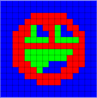
Above is an RGB image with a pixel color distribution of roughly the following:

red = 30%
green = 10%
blue = 60%

Therefore, if we were to randomly sample a pixel color from the image ('im1'), we would have the following probabilities of sampling each color:

P(R|im1) = .3
P(G|im1) = .1
P(B|im1) = .6

Given the following probabilities of two more RGB images with the same number of pixels as im1, solve (a), (b), and (c). (Note: we assume for this problem that pixels are sampled with replacement.)

P(R|im1) = .3	P(R|im2) = .8	P(R|im3) = .4
P(G|im1) = .1	P(G|im2) = .1	P(G|im3) = .2     } where R = red pixel sampled, etc, and im1 = pixel sampled is in image 1, etc.
P(B|im1) = .6	P(B|im2) = .1	P(B|im3) = .4

(a) Assuming that we have an equal probability of sampling a pixel from each image, what is the probability that a sampled red
    pixel came from image 3? 

(b) Now, assume that after the first pixel is sampled, our remaining pixel samples must come from the same image as the first
    pixel.  Given that we first sampled a red pixel, then a green and blue, what is the probability that we have been sampling
    from image 1?

(c) Given the same {R,G,B} scenario as (b), and where pixels after the first must come from the same image, what is the
    probability that our next (fourth) pixel sampled is red?

Solution

(a)

We have been asked to find P(im3|R):

$ P(im3|R) = \frac{P(im3 \cap R)}{P(R)} $ from conditional probability $ = \frac{P(im3)P(R|im3)}{P(R)} $ from Bayes' rule

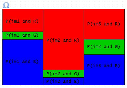
Because the numerators of the previous equation are both given, we are only left to find P(R). Since the sample space is partitioned into disjoint subsets im1, im2, and im3 (see graphic below), we can use the law of total probability:

$ P(R) = \sum_{i=1}^{3} P(im_i)P(R|im_i) = \frac{1}{3}(.3 + .8 + .4) = .5 $

$ \therefore P(im3|R) = \frac{(\frac{1}{3})(.4)}{.5} = \frac{.4}{1.5} $

(b)

We know that once an image has been sampled from, future pixel color order does not matter since pixels are sampled with replacement. However, it's crucial to note for (b) and (c) that order does matter for the first pixel (when the image number is not yet known).

The naive calculation would be $ P(R|im_i)*P(G|im_i)*P(B|im_i) $. However, what we really want is $ P(im_i|R)*P(G|im_i)*P(B|im_i) $. To see the difference, consider:

$ P(R|im_3) = .4 \neq P(im_3|R) = \frac{.4}{1.5} $

So first we need to determine the probability that the first (red) pixel was sampled from image 1. Using the same method as in (a):

$ P(im1|R) = \frac{(\frac{1}{3})(.3)}{.5} = \frac{.3}{1.5} = \frac{1}{5} $

(c)

For (b) and (c) it's important to realize that there is independence of subsequent pixel samplings within an image (intra-image, "locally"). However, if the image sampled from is not known, a sequence but dependence of subsequent pixel samplings between images (inter-image, "globally").

 (Note that because pixels are not removed from the image after being sampled, the order of pixels sampled
    after the first pixel does not matter.)

Back to first bonus point opportunity, ECE302 Spring 2013