(New page: = Linearity = There are three definitions we discussed in class for linearity. <u></u><u>Definition 1</u> <u></u>A system is called linear if for any constants <\math> a,b = \epsilon <...) |
|||
| (10 intermediate revisions by one other user not shown) | |||
| Line 1: | Line 1: | ||
| − | = Linearity = | + | [[Category:bonus point project]] |
| + | === Linearity === | ||
| − | + | == Theory == | |
| − | + | There are three definitions we discussed in class for linearity. | |
| − | <u></u>A system is called linear if for any constants < | + | <u></u>'''<u>Definition 1</u>''' |
| + | |||
| + | <u></u>A system is called '''linear''' if for any constants <math>a,b\in </math> ''all complex numbers'' and for any input signals <span class="texhtml">''x''<sub>1</sub>(''t''),''x''<sub>2</sub>(''t'')</span> with response <span class="texhtml">''y''<sub>1</sub>(''t''),''y''<sub>2</sub>(''t'')</span>, respectively, the system's response to <span class="texhtml">''ax''<sub>1</sub>(''t'') + ''b''x''<sub>2</sub>(''t'')'' ''is ''ay''<sub>1</sub>(''t'') + ''b''y''<sub>2</sub>(''t''). </span> | ||
| + | |||
| + | '''<u>Definition 2</u>''' | ||
| + | |||
| + | If | ||
| + | |||
| + | <math> x_1(t) \rightarrow \begin{bmatrix} system \end{bmatrix} \rightarrow y_1(t) </math> | ||
| + | |||
| + | <math> x_2(t) \rightarrow \begin{bmatrix} system \end{bmatrix} \rightarrow y_2(t) </math> | ||
| + | |||
| + | then | ||
| + | |||
| + | <math> ax_1(t) + bx_2(t) \rightarrow \begin{bmatrix} system \end{bmatrix} \rightarrow ay_1(t) + by_2(t) </math> | ||
| + | |||
| + | for any <math>a,b\in </math> ''all complex numbers'', any <span class="texhtml">''x''<sub>1</sub>(''t''),''x''<sub>2</sub>(''t'')</span> then we say the system is '''linear'''. | ||
| + | |||
| + | '''<u>Definition 3</u>''' | ||
| + | |||
| + | <u></u>[[Image:Slide1.jpg]]<br> | ||
| + | |||
| + | == Applications == | ||
| + | |||
| + | Linearity can be used to simplify the Fourier transform. Integration and differentiation are also linear. Once a non-linear system is made linear, complex systems are easier to model mathematically. True linear systems are virtually unknown in the real world, but over a small range of variables, systems can be modeled as linear. | ||
| + | |||
| + | <br> | ||
| + | |||
| + | <br> | ||
| + | |||
| + | <br> | ||
Latest revision as of 09:50, 6 May 2012
Linearity
Theory
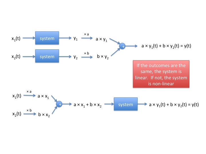
There are three definitions we discussed in class for linearity.
Definition 1
A system is called linear if for any constants $ a,b\in $ all complex numbers and for any input signals x1(t),x2(t) with response y1(t),y2(t), respectively, the system's response to ax1(t) + bx2(t) is ay1(t) + by2(t).
Definition 2
If
$ x_1(t) \rightarrow \begin{bmatrix} system \end{bmatrix} \rightarrow y_1(t) $
$ x_2(t) \rightarrow \begin{bmatrix} system \end{bmatrix} \rightarrow y_2(t) $
then
$ ax_1(t) + bx_2(t) \rightarrow \begin{bmatrix} system \end{bmatrix} \rightarrow ay_1(t) + by_2(t) $
for any $ a,b\in $ all complex numbers, any x1(t),x2(t) then we say the system is linear.
Definition 3
Applications
Linearity can be used to simplify the Fourier transform. Integration and differentiation are also linear. Once a non-linear system is made linear, complex systems are easier to model mathematically. True linear systems are virtually unknown in the real world, but over a small range of variables, systems can be modeled as linear.


