| (8 intermediate revisions by 2 users not shown) | |||
| Line 1: | Line 1: | ||
| − | == Homework 6 Solution == | + | == ECE438 [[Hw6ECE438F10|Homework 6]] Solution == |
Q1. | Q1. | ||
| Line 73: | Line 73: | ||
Flow diagram of FFT: | Flow diagram of FFT: | ||
| − | [[Image:diagramFFT1.jpg]] | + | [[Image:diagramFFT1.jpg]] |
Analytical Expressions: | Analytical Expressions: | ||
| Line 99: | Line 99: | ||
Flow diagram of FFT: | Flow diagram of FFT: | ||
| − | [[Image:diagramFFT2.jpg]] | + | [[Image:diagramFFT2.jpg]] |
Analytical Expressions: | Analytical Expressions: | ||
| Line 108: | Line 108: | ||
&\text{Change variable n=3m+l, m=0,1; l=0,1,2 } \\ | &\text{Change variable n=3m+l, m=0,1; l=0,1,2 } \\ | ||
X_N(k)&=\sum_{l=0}^{2}\sum_{m=0}^{1}x(3m+l)e^{-\frac{j2\pi k(3m+l)}{N}} \\ | X_N(k)&=\sum_{l=0}^{2}\sum_{m=0}^{1}x(3m+l)e^{-\frac{j2\pi k(3m+l)}{N}} \\ | ||
| − | &=\sum_{l=0}^{2}e^{-\frac{j2\pi kl}{N}}\sum_{m=0}^{1}x(3m+l)e^{-\frac{j2\pi km | + | &=\sum_{l=0}^{2}e^{-\frac{j2\pi kl}{N}}\sum_{m=0}^{1}x(3m+l)e^{-\frac{j2\pi km}{N/3}} \\ |
&=\sum_{l=0}^{2}W_N^{kl}X_l(k) \text{ ,k=0,1,...,N-1 } | &=\sum_{l=0}^{2}W_N^{kl}X_l(k) \text{ ,k=0,1,...,N-1 } | ||
\end{align} | \end{align} | ||
| Line 128: | Line 128: | ||
Flow Diagram: | Flow Diagram: | ||
| − | [[Image:HW6_Q4_FFT.jpg]] | + | [[Image:HW6_Q4_FFT.jpg]] |
<math>5120=5*1024=5*2^{10}</math> So we can split the 5120-point DFT into 5 1024-point DFTs using decimation-in-time and compute the 1024-point DFT using the subroutine of radix 2 FFT. | <math>5120=5*1024=5*2^{10}</math> So we can split the 5120-point DFT into 5 1024-point DFTs using decimation-in-time and compute the 1024-point DFT using the subroutine of radix 2 FFT. | ||
| Line 139: | Line 139: | ||
&\text{Change variable n=5m+l, m=0,1,...,1023; l=0,1,...,4 } \\ | &\text{Change variable n=5m+l, m=0,1,...,1023; l=0,1,...,4 } \\ | ||
X^{(5120)}(k)&=\sum_{l=0}^{4}\sum_{m=0}^{1023}x(5m+l)e^{-\frac{j2\pi k(5m+l)}{5120}} \\ | X^{(5120)}(k)&=\sum_{l=0}^{4}\sum_{m=0}^{1023}x(5m+l)e^{-\frac{j2\pi k(5m+l)}{5120}} \\ | ||
| − | &=\sum_{l=0}^{4}e^{-\frac{j2\pi kl}{5120}}\sum_{m=0}^{1023}x(5m+l)e^{-\frac{j2\pi km | + | &=\sum_{l=0}^{4}e^{-\frac{j2\pi kl}{5120}}\sum_{m=0}^{1023}x(5m+l)e^{-\frac{j2\pi km}{1024}} \\ |
&=\sum_{l=0}^{4}W_{5120}^{kl}X_l^{(1024)}(k) \text{ ,k=0,1,...,5119 } | &=\sum_{l=0}^{4}W_{5120}^{kl}X_l^{(1024)}(k) \text{ ,k=0,1,...,5119 } | ||
\end{align} | \end{align} | ||
| Line 212: | Line 212: | ||
&x(n)=\frac{1}{N}\sum_{k=0}^{N-1}X(k)e^{j\frac{j2\pi kn}{N}} \\ | &x(n)=\frac{1}{N}\sum_{k=0}^{N-1}X(k)e^{j\frac{j2\pi kn}{N}} \\ | ||
&\text{Switch n and k} \\ | &\text{Switch n and k} \\ | ||
| − | \Leftrightarrow &x(k)=\frac{1}{N}\sum_{ | + | \Leftrightarrow &x(k)=\frac{1}{N}\sum_{n=0}^{N-1}X(n)e^{j\frac{j2\pi kn}{N}} \\ |
| − | \Leftrightarrow &Nx(-k)=\sum_{ | + | \Leftrightarrow &Nx(-k)=\sum_{n=0}^{N-1}X(n)e^{-j\frac{j2\pi kn}{N}}=\text{ DFT of }X(n) |
\end{align} | \end{align} | ||
</math> | </math> | ||
| Line 227: | Line 227: | ||
Suppose a and b are constant, l is a arbitrary integer. Denote <math>y[n]=\mathcal{T}\{ x[n]\} </math> | Suppose a and b are constant, l is a arbitrary integer. Denote <math>y[n]=\mathcal{T}\{ x[n]\} </math> | ||
| − | a) | + | a) Yes |
| + | |||
| + | Since | ||
<math> | <math> | ||
| Line 237: | Line 239: | ||
</math> | </math> | ||
| − | The system is linear | + | The system is linear. |
<math>\mathcal{T}\{x[n-l]\}=x[n-l+1]+x[n-l-1]</math> | <math>\mathcal{T}\{x[n-l]\}=x[n-l+1]+x[n-l-1]</math> | ||
<math>y[n-l]=x[n-l+1]+x[n-l-1]</math> | <math>y[n-l]=x[n-l+1]+x[n-l-1]</math> | ||
| + | |||
| + | Since | ||
| + | |||
| + | <math>\mathcal{T}\{x[n-l]\}=y[n-l]</math> | ||
The system is time invariant. | The system is time invariant. | ||
| Line 247: | Line 253: | ||
As a result, the system is LTI. | As a result, the system is LTI. | ||
| − | b) | + | b) No |
| + | |||
| + | Since | ||
<math> | <math> | ||
| Line 257: | Line 265: | ||
</math> | </math> | ||
| − | The system is linear | + | The system is linear. |
| + | |||
| + | <math>\mathcal{T}\{x[n-l]\}=x[n-l-1]+x[1-n-l]</math> | ||
| + | |||
| + | <math>y[n-l]=x[n-l+1]+x[1-n+l]</math> | ||
| + | |||
| + | Since | ||
| + | |||
| + | <math>\mathcal{T}\{x[n-l]\}\ne y[n-l]</math> | ||
| + | |||
| + | The system is time variant. | ||
| + | |||
| + | As a result, the system is not LTI. | ||
| + | |||
| + | c) Yes | ||
| + | |||
| + | Since | ||
| + | |||
| + | <math> | ||
| + | \begin{align} | ||
| + | \mathcal{T}\{ax_1[n]+bx_2[n]\}&=(ax_1[n]+bx_2[n])*(u[n+3]-u[n-3]) \\ | ||
| + | &=\sum_{k=-\infty}^{\infty}(ax_1[n-k]+bx_2[n-k])(u[k+3]-u[k-3]) \\ | ||
| + | &=a\sum_{k=-\infty}^{\infty}x_1[n-k](u[k+3]-u[k-3])+b\sum_{k=-\infty}^{\infty}x_2[n-k](u[k+3]-u[k-3]) \\ | ||
| + | &=a\mathcal{T}\{x_1[n]\}+b\mathcal{T}\{x_2[n]\} | ||
| + | \end{align} | ||
| + | </math> | ||
| + | |||
| + | The system is linear. | ||
| + | |||
| + | <math>\mathcal{T}\{x[n-l]\}=x[n-l]*(u[n-l+3]-u[n-l-3])</math> | ||
| + | |||
| + | <math>y[n-l]=x[n-l]*(u[n-l+3]-u[n-l-3])</math> | ||
| + | |||
| + | Since | ||
| + | |||
| + | <math>\mathcal{T}\{x[n-l]\}=y[n-l]</math> | ||
| + | |||
| + | The system is time invariant. | ||
| + | |||
| + | As a result, the system is LTI. | ||
----------------------- | ----------------------- | ||
[[2010_Fall_ECE_438_Boutin|Back to Course Homepage]] | [[2010_Fall_ECE_438_Boutin|Back to Course Homepage]] | ||
[[Hw6ECE438F10|Back to Homework 6 Questions]] | [[Hw6ECE438F10|Back to Homework 6 Questions]] | ||
Latest revision as of 16:44, 23 October 2011
ECE438 Homework 6 Solution
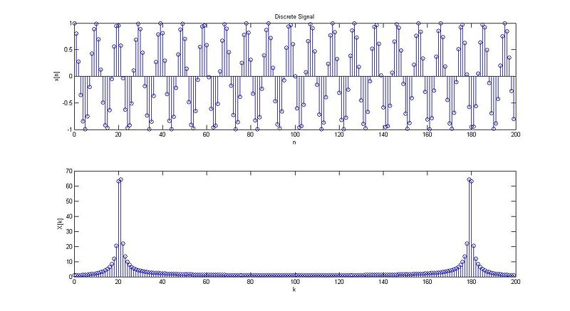
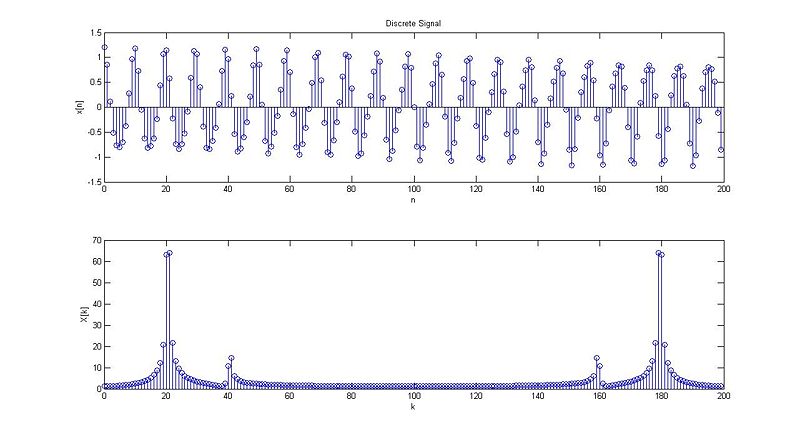
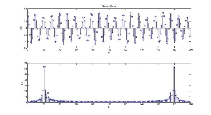
Q1.
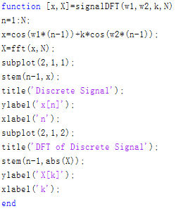
Matlab code:
Assign the value of parameters and then call the function signalDFT
For example, in case 6 type following command in the command window of Matlab:
N=20;
w1=0.62831853;
k=0.2;
w2=0.79168135;
[x,X]=signal(w1,w2,k,N);
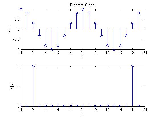
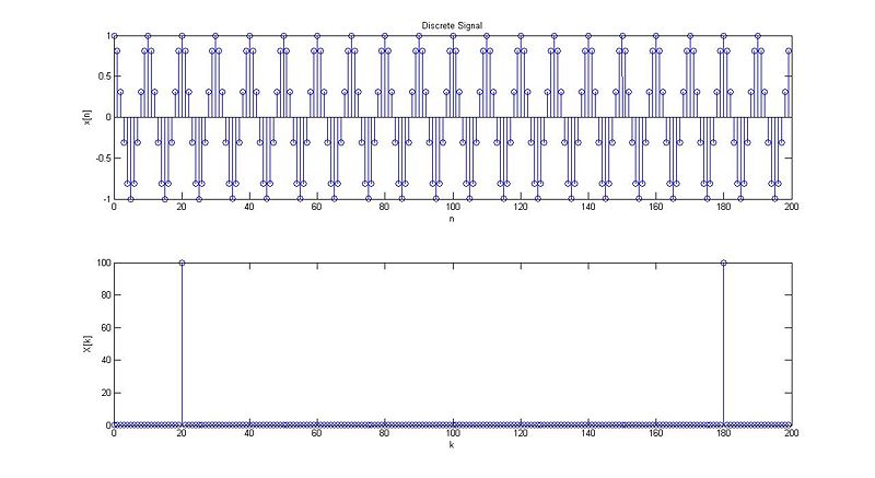
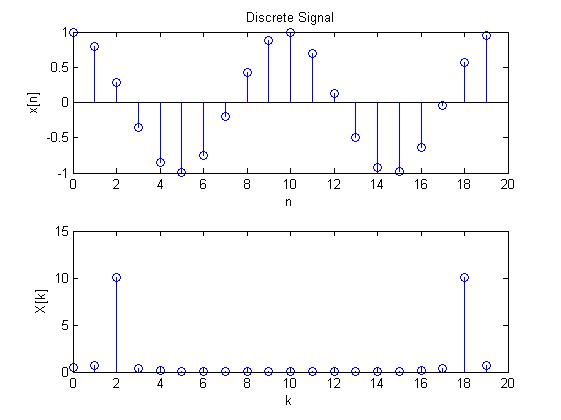
Plot result:
case 1:
case 2:
case 3:
case 4:
case 5:
case 6:
Q2.
Recall the definition of DFT:
$ X[k]=\sum_{n=0}^{N-1} x[n]e^{-j2\pi k/N} $
In this question N=8
If we use summation formula to compute DFT, for each k, we need N times complex multiplications and N times complex additions.
In total, we need N*N=64 times of complex multiplications and N*(N-1)=56 times of complex additions.
In decimation-in-time FFT algorithm, we keep on decimating the number of points by 2 until we get 2 points DFT. At most, we can decimate $ v=log_2 N $ times. As a result, we get v levels of DFT. For each level, we need N/2 times of complex multiplications and N times of complex additions.
In total, we need $ \frac{N}{2}log_2 N=12 $ times of complex multiplications and $ Nlog_2 N=24 $ times of complex additions.
Q3.
Denote N is the points number of the input signal's DFT. Then N=6.
1) The normal DFT algorithm: If we use summation formula to compute DFT, according to the analysis of Q2. We need N*N=36 times of complex multiplications and N*(N-1)=30 times of complex additions.
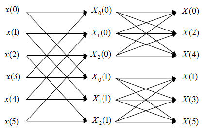
Flow diagram of FFT:
Analytical Expressions:
$ \begin{align} X_N(k)&=\sum_{n=0}^{N-1} x(n)e^{-\frac{j2\pi kn}{N}} \\ &\text{Change variable n=2m+l, m=0,1,2; l=0,1 } \\ X_N(k)&=\sum_{l=0}^{1}\sum_{m=0}^{2}x(2m+l)e^{-\frac{j2\pi k(2m+l)}{N}} \\ &=\sum_{l=0}^{1}e^{-\frac{j2\pi kl}{N}}\sum_{m=0}^{2}x(2m+l)e^{-\frac{j2\pi km)}{N/2}} \\ &=\sum_{l=0}^{1}W_N^{kl}X_l(k) \text{ ,k=0,1,...,N-1 } \end{align} $
In this FFT algorithm, the computing of DFT is divided into two levels. First, we compute two 3-point DFT, which are DFT of even and odd points.
In this step we need 4 times of complex multiplications and 6 times of complex additions for each 3-point DFT. Since we have to do this twice, we need 4*2=8 times of complex multiplications and 6*2=12 times of complex additions.
Second, we compute the final DFT by combing the first level result. According to the analysis of Q2, we need N/2=3 times of complex multiplications and N=6 times of complex additions.
In total, we need 8+3=11 times of complex multiplications and 12+6=18 times of complex additions.
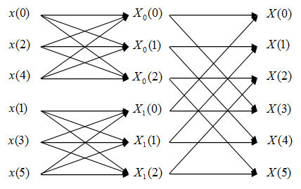
2)
Flow diagram of FFT:
Analytical Expressions:
$ \begin{align} X_N(k)&=\sum_{n=0}^{N-1} x(n)e^{-\frac{j2\pi kn}{N}} \\ &\text{Change variable n=3m+l, m=0,1; l=0,1,2 } \\ X_N(k)&=\sum_{l=0}^{2}\sum_{m=0}^{1}x(3m+l)e^{-\frac{j2\pi k(3m+l)}{N}} \\ &=\sum_{l=0}^{2}e^{-\frac{j2\pi kl}{N}}\sum_{m=0}^{1}x(3m+l)e^{-\frac{j2\pi km}{N/3}} \\ &=\sum_{l=0}^{2}W_N^{kl}X_l(k) \text{ ,k=0,1,...,N-1 } \end{align} $
In this FFT algorithm, the computing of DFT is still divided into two levels. However, we will first compute three 2 points DFT, which are DFT of the first half points and the second half points. According to analysis of Q2, we need N/2=3 times of complex multiplications and N=6 times of complex additions.
Second, we compute the two 3 points DFT using first level result. we need 4 times of complex multiplications and 6 times of complex additions for each 3-point DFT. Since we have to do this twice, we need 4*2=8 times of complex multiplications and 6*2=12 times of complex additions.
In total, we need 3+8=11 times of complex multiplications and 6+12=18 times of complex additions.
Notice that the output sequences of DFT of 2) is different from 1).
Compare 1) and 2), both methods have the same amount of complex operations.
Q4.
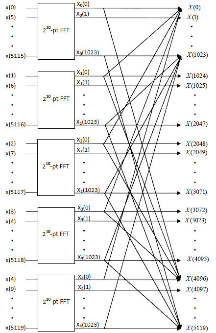
Flow Diagram:
$ 5120=5*1024=5*2^{10} $ So we can split the 5120-point DFT into 5 1024-point DFTs using decimation-in-time and compute the 1024-point DFT using the subroutine of radix 2 FFT.
Analytical expression:
$ \begin{align} X^{(5120)}(k)&=\sum_{n=0}^{5119} x(n)e^{-\frac{j2\pi kn}{5120}} \\ &\text{Change variable n=5m+l, m=0,1,...,1023; l=0,1,...,4 } \\ X^{(5120)}(k)&=\sum_{l=0}^{4}\sum_{m=0}^{1023}x(5m+l)e^{-\frac{j2\pi k(5m+l)}{5120}} \\ &=\sum_{l=0}^{4}e^{-\frac{j2\pi kl}{5120}}\sum_{m=0}^{1023}x(5m+l)e^{-\frac{j2\pi km}{1024}} \\ &=\sum_{l=0}^{4}W_{5120}^{kl}X_l^{(1024)}(k) \text{ ,k=0,1,...,5119 } \end{align} $
Direct computation requires N*N=5120*5120=26214400 times of complex multiplications and N*(N-1)=5120*5119=26209280 times of complex additions.
Using FFT we first perform five 1024-point FFTs, which each require $ \frac{N}{2}log_2 N=512*10=5120 $ complex multiplications and $ Nlog_2 N=1024*10=10240 $ complex additions.
To calculate each of the 5120 final output of the 5120 DFT, we have to perform 5 complex multiplications and 4 complex additions. So we need 5120*5= 25600 times of complex multiplications and 5120*4=20480 times of complex additions.
For the FFT based method we have a total of 5120+25600=30720 complex multiplications and 10240+20480=30720 complex addtions.
By compare the two methods, we see that FFT based method is far more efficient than the direct computation.
Q5.
First, consider obtaining DFT from a finite duration signal.
$ \bar x[n] $ is a discrete finite signal with duration N.
i.e. $ \bar x[n]=0 \text{ when n} \ge N $
$ \bar \mathcal{X}(\omega) $ is the DTFT of $ \bar x[n] $
$ x_p[n] $ is the periodical extension of $ \bar x[n] $ with a period P
i.e. $ x_p[n]=\sum_{l=-\infty}^{\infty}\bar x[n+lP] $
Then we can compute DFT by $ X[k]=\bar \mathcal{X}(k\frac{2\pi}{P})=\sum_{n=0}^{P-1}x[n]e^{-j\frac{2\pi kn}{P}} \text{ k=0,1,...,P-1} $
In order to fully construct DTFT from DFT, we must have $ P\ge N $
Consider reconstruction DTFT from DFT.
Observe
$ \begin{align} \bar \mathcal{X}(\omega)&=\sum_{n=-\infty}^{\infty}\bar x[n]e^{-j\omega n} \\ &=\sum_{n=0}^{N-1}\bar x[n]e^{-j\omega n} \text{ ,Since } \bar x \text{ has finite duration N} \\ &=\sum_{n=0}^{N-1}x_P[n]e^{-j\omega n} \text{ ,Since } P\ge N \\ &=\sum_{n=0}^{N-1}(\frac{1}{N}\sum_{k=0}^{N-1}X(k)e^{\frac{j2\pi kn}{N}})e^{-j\omega n} \\ &=\sum_{k=0}^{N-1}X(k)\sum_{n=0}^{N-1}\frac{1}{N}e^{-j(\omega-\frac{j2\pi k}{N})n} \end{align} $
$ \text{Denote } P(\omega)=\frac{1}{N}\sum_{n=0}^{N-1}e^{-j(\omega-\frac{j2\pi k}{N})n} $
$ \text{Then } P(\omega)=\left\{\begin{array}{ll}1, & \text{ if }\omega =0,\pm 2\pi,...\\ \frac{1}{N}e^{\frac{-j\omega (N-1)}{2}}\frac{sin(\frac{\omega N}{2})}{sin(\frac{\omega}{2})}, & \text{else.}\end{array} \right. \ $
So DTFT can be fully constructed by
$ \bar \mathcal{X}(\omega)=\sum_{k=0}^{N-1}X(k)P(\omega -\frac{2\pi k}{N}) $
Note: In practice, we often choose P exactly the same as N
Q6.
The Duality Property of DFT is descriped below:
$ \text{If the DFT of }x[n]\text{ is denoted as }X(k)\text{ with a length of N} $
$ \text{Then the DFT of }X(n)\text{ is }Nx(-k) $
Derivation:
$ \begin{align} &x(n)=\frac{1}{N}\sum_{k=0}^{N-1}X(k)e^{j\frac{j2\pi kn}{N}} \\ &\text{Switch n and k} \\ \Leftrightarrow &x(k)=\frac{1}{N}\sum_{n=0}^{N-1}X(n)e^{j\frac{j2\pi kn}{N}} \\ \Leftrightarrow &Nx(-k)=\sum_{n=0}^{N-1}X(n)e^{-j\frac{j2\pi kn}{N}}=\text{ DFT of }X(n) \end{align} $
Conclusion:
if $ x(n)\xrightarrow{DFT} X(k) $
then $ X(n)\xrightarrow{DFT} Nx(-k) $
Q7.
Suppose a and b are constant, l is a arbitrary integer. Denote $ y[n]=\mathcal{T}\{ x[n]\} $
a) Yes
Since
$ \begin{align} \mathcal{T}\{ax_1[n]+bx_2[n]\}&=ax_1[n+1]+bx_2[n+1]+ax_1[n-1]+bx_2[n-1] \\ &=ax_1[n+1]+ax_1[n-1]+bx_2[n+1]+bx_2[n-1] \\ &=a\mathcal{T}\{x_1[n]\}+b\mathcal{T}\{x_2[n]\} \end{align} $
The system is linear.
$ \mathcal{T}\{x[n-l]\}=x[n-l+1]+x[n-l-1] $
$ y[n-l]=x[n-l+1]+x[n-l-1] $
Since
$ \mathcal{T}\{x[n-l]\}=y[n-l] $
The system is time invariant.
As a result, the system is LTI.
b) No
Since
$ \begin{align} \mathcal{T}\{ax_1[n]+bx_2[n]\}&=ax_1[n-1]+bx_2[1-n]+ax_1[n-1]+bx_2[1-n] \\ &=ax_1[n-1]+ax_1[1-n]+bx_2[n-1]+bx_2[1-n] \\ &=a\mathcal{T}\{x_1[n]\}+b\mathcal{T}\{x_2[n]\} \end{align} $
The system is linear.
$ \mathcal{T}\{x[n-l]\}=x[n-l-1]+x[1-n-l] $
$ y[n-l]=x[n-l+1]+x[1-n+l] $
Since
$ \mathcal{T}\{x[n-l]\}\ne y[n-l] $
The system is time variant.
As a result, the system is not LTI.
c) Yes
Since
$ \begin{align} \mathcal{T}\{ax_1[n]+bx_2[n]\}&=(ax_1[n]+bx_2[n])*(u[n+3]-u[n-3]) \\ &=\sum_{k=-\infty}^{\infty}(ax_1[n-k]+bx_2[n-k])(u[k+3]-u[k-3]) \\ &=a\sum_{k=-\infty}^{\infty}x_1[n-k](u[k+3]-u[k-3])+b\sum_{k=-\infty}^{\infty}x_2[n-k](u[k+3]-u[k-3]) \\ &=a\mathcal{T}\{x_1[n]\}+b\mathcal{T}\{x_2[n]\} \end{align} $
The system is linear.
$ \mathcal{T}\{x[n-l]\}=x[n-l]*(u[n-l+3]-u[n-l-3]) $
$ y[n-l]=x[n-l]*(u[n-l+3]-u[n-l-3]) $
Since
$ \mathcal{T}\{x[n-l]\}=y[n-l] $
The system is time invariant.
As a result, the system is LTI.

