| Line 53: | Line 53: | ||
The Chernoff bound is found by analytically or numerically minimizing <math>e^{-f(\beta)}</math>, therefore optimization is now in the one dimensional β space. | The Chernoff bound is found by analytically or numerically minimizing <math>e^{-f(\beta)}</math>, therefore optimization is now in the one dimensional β space. | ||
[[Image:Error.jpg]] | [[Image:Error.jpg]] | ||
| + | |||
| + | Now consider a special case where : <math>\Sigma_1 = \Sigma_2 =: \Sigma</math> | ||
| + | |||
| + | <math>f(\beta) = \beta (1-\beta){(\mu_2 - \mu_1)^T} \Sigma^{-1}(\mu_2 - \mu_1)</math> | ||
| + | |||
| + | <math>\frac {df(\beta)}{d\beta} = \frac {1-2\beta}{2}{(\mu_2 - \mu_1)^T} \Sigma^{-1}(\mu_2 - \mu_1)= 0</math> | ||
| + | |||
| + | <math> \Leftrightarrow \beta = \frac {1}{2}</math> | ||
| + | therefore Bhattacharyya Bound is optimum in this case. | ||
Revision as of 14:32, 9 May 2010
Classic central limit Thm (Second Fundamental probabilistic):
"The distribution of the average of a large number of samples from a distribution tends to be normal"
let X1,X2,...,Xn be n independent and identically distributed variables (i.i.d) with finite mean $ \mu $ and finite variance $ \sigma^2>0 $.Then as n increases the distribution of $ \Sigma_{i=1}^n \frac{X_i} {n} $ approaches $ N(\mu,\frac {\sigma^2}{n}) $.
More precisely the random variable $ Z_n = \frac{\Sigma_{i=1}^n X_i - n \mu}{\sigma \sqrt{n}} $ has $ P(Z_n)\longrightarrow N(0,1) $ when $ n \longrightarrow \infty $
More generalization of central limit Thm.
let X1,X2,...,Xn be n independent variables
Xi has mean $ \mu_i $ and finite variance $ \sigma^2 > 0 $ ,i=1,2,...,n
Then $ Z_n = \frac{\Sigma_{i=1}^n X_i - \Sigma_{i=1}^n \mu_i} {\sqrt{\Sigma_{i=1}^n \sigma^2}} $ has $ P(Z_n)\longrightarrow N(\mu ,\Sigma) $ when $ n \longrightarrow \infty $
Error bounds for Bayes decision rule:
As we know Bayes decision rule guarantees the lowest average error rate; It Does not tell what the probability of error actually is. Therefore people try to find upper bounds for that: Chernoff and Bhattacharyya bounds
$ P(error)=\int_{R^n} p(error,x)dx = \int_{R^n} p(error|x)p(x)dx $
in two class case we have:
$ p(error|x) = min \{ p(\omega_1|x) , p(\omega_2|x) \} $ $ \Rightarrow P(error)= \int_{R^n}min\{p(\omega_1|x),p(\omega_2|x)\} p(x)dx $
as we know from Lemma: $ min \{a,b\}\leq a^\beta b^ {1-\beta} $, $ \forall a,b \geq 0 , \forall \beta s.t 0 \leq\beta\leq 1 $
$ P(error)\leq \int_{R^n} p(\omega_1 |x)^\beta p(\omega_2 |x)^{1-\beta} p(x) dx $ , $ \forall 0 \leq \beta \leq 1 $
$ P(error)\leq \int_{R^n} ({\frac {p(x|\omega)P(\omega_1)}{p(x)}})^\beta ({\frac {p(x|\omega_2)P(\omega_2)}{p(x)}})^{1-\beta} p(x) dx $ , $ \forall 0 \leq \beta \leq 1 $
$ P(error)\leq P(\omega_1) ^\beta P(\omega_2)^ https://kiwi.ecn.purdue.edu/rhea/skins/common/images/button_math.png{1-\beta} \int_{R^n} p(x|\omega_1)^\beta p(x|\omega_2)^{1-\beta} dx =: \varepsilon_\beta $ , $ \forall 0 \leq \beta \leq 1 $
The lower bound $ S:= min\varepsilon_\beta $ , $ \beta \in [0,1] $is an upper bound for P(error).
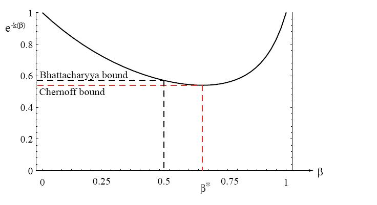
S is called "Chernoff Bound" and $ \varepsilon_{1/2} $ is called "Bhattacharyya Bound"
$ \varepsilon_{1/2}= \sqrt{P(\omega_1)P(\omega_2)} \int_{R^n} \sqrt{p(x|\omega_1)p(x|\omega_2)} dx = e^{-f(1/2)} \sqrt {P(\omega_1)P(\omega_2)} $
$ \varepsilon_\beta = P(\omega_1) ^\beta P(\omega_2)^ {1-\beta} \int_{R^n} p(x|\omega_1)^\beta p(x|\omega_2)^{1-\beta} dx = e^{-f(\beta)} P(\omega_1)^\beta P(\omega_2)^ {1-\beta} $
Here $ f(1/2) $ is "Bhattacharyya distance" and $ f(\beta) $ is "Chernof distance"
Especial case: Bounds for Gaussian density:
$ f(\beta)= {\frac{ \beta (1- \beta)}{2}} {(\mu_2 - \mu_1)^T} [ \beta \Sigma_1 + (1- \beta) \Sigma_2]^{-1} (\mu_2-\mu_1) + \frac {1}{2} ln{\frac {|\beta \Sigma_1 + (1-\beta) \Sigma_2|}{|\Sigma_1|^\beta |\Sigma_2|^ {1-\beta}}} $
$ f(1/2)=\frac{1}{8} (\mu_2 - \mu_1)^T [\frac {\Sigma_1 + \Sigma_2} {2}]^{-1} (\mu_2 - \mu_1) + \frac {1} {2} ln \frac {[\frac {\Sigma_1 + \Sigma_2} {2}]} {\sqrt {|\Sigma_1| |\Sigma_2|}} $
The Chernoff bound is found by analytically or numerically minimizing $ e^{-f(\beta)} $, therefore optimization is now in the one dimensional β space.

Now consider a special case where : $ \Sigma_1 = \Sigma_2 =: \Sigma $
$ f(\beta) = \beta (1-\beta){(\mu_2 - \mu_1)^T} \Sigma^{-1}(\mu_2 - \mu_1) $
$ \frac {df(\beta)}{d\beta} = \frac {1-2\beta}{2}{(\mu_2 - \mu_1)^T} \Sigma^{-1}(\mu_2 - \mu_1)= 0 $
$ \Leftrightarrow \beta = \frac {1}{2} $ therefore Bhattacharyya Bound is optimum in this case.

