(New page: See also: [Fisher Linear Discriminant] In this derivation, we assume the dimension of the space being projected to, k, is k=1. We attempt to find a linear projection (line that passes th...) |
|||
| Line 7: | Line 7: | ||
**sorry, I did not realize that this image would change while I was working on [Lecture 11] I changed the name of the other image so whoever has the original animation can put it back** | **sorry, I did not realize that this image would change while I was working on [Lecture 11] I changed the name of the other image so whoever has the original animation can put it back** | ||
| − | + | [[Image:projection_OldKiwi.gif]] | |
| − | + | Assume <math>y_1,..., y_{d_1}</math> belongs to Class 1 and <math>y_{d_1+1}</math>,..., <math>y_d</math> belongs to Class 2. | |
| − | + | ||
| − | + | ||
| − | + | ||
| − | + | ||
| − | + | ||
| − | + | ||
| − | + | ||
| − | + | ||
| − | Assume <math>y_1 | + | |
Consider the sample mean of the projected data for each class | Consider the sample mean of the projected data for each class | ||
| Line 24: | Line 15: | ||
<math>\tilde{m_1} = \frac{1}{d_1} \sum_{i=1}^{d_1} \pi(y_i) = \frac{1}{d_1}\sum_{i=1}^{d_1} \vec{w} \cdot y_i</math>, if <math>||\omega || =1</math> | <math>\tilde{m_1} = \frac{1}{d_1} \sum_{i=1}^{d_1} \pi(y_i) = \frac{1}{d_1}\sum_{i=1}^{d_1} \vec{w} \cdot y_i</math>, if <math>||\omega || =1</math> | ||
| − | **Observation:** <math>m1 = \vec{w} \frac{1}{d_1} \sum_{i=1}^{d_1} y_i</math>, which is the projection of the sample mean for Class 1. | + | **Observation:** <math>m1 = \vec{w} \frac{1}{d_1} \sum_{i=1}^{d_1} y_i</math>, which is the projection of the sample mean for Class 1. |
Also, <math>\tilde{m_2} = \frac{1}{d-d_1}\sum_{i=d_1+1}^{d} \vec{w} \cdot y_i = \vec{w} \cdot m_2</math> . | Also, <math>\tilde{m_2} = \frac{1}{d-d_1}\sum_{i=d_1+1}^{d} \vec{w} \cdot y_i = \vec{w} \cdot m_2</math> . | ||
| Line 43: | Line 34: | ||
Need to fix <math>|| \omega || = 1</math> , resulting in a Constrained Optimization Problem. | Need to fix <math>|| \omega || = 1</math> , resulting in a Constrained Optimization Problem. | ||
| − | |||
| − | |||
| − | |||
| − | |||
| − | |||
| − | |||
| − | |||
| − | |||
| − | |||
| − | |||
By dividing by <math>\tilde{S_1}^2 + \tilde{S_2}^2</math> we demand that <math>\vec{w} \cdot (m_1 - m_2)</math> be large in comparison with the scatter. This allows you to bypass the coordinate scale problem because <math>J(\vec{w})</math> is independent of <math>\omega</math>. | By dividing by <math>\tilde{S_1}^2 + \tilde{S_2}^2</math> we demand that <math>\vec{w} \cdot (m_1 - m_2)</math> be large in comparison with the scatter. This allows you to bypass the coordinate scale problem because <math>J(\vec{w})</math> is independent of <math>\omega</math>. | ||
.. |eq2| image:: tex | .. |eq2| image:: tex | ||
| − | + | :alt: tex: |\tilde{m_1} - \tilde{m_2}|^2 = | w(m_1 - m_2)|^2 = |w|^2 | \frac{w}{|w|}(m_1-m_2)|^2 | |
.. |eq3| image:: tex | .. |eq3| image:: tex | ||
| − | + | :alt: tex: \tilde{S_1}^2 = \sum (\vec{w}(y_i - m_1))^2 = |w|^2 \sum (\frac{w}{|W|} (y_i - m_1))^2 | |
.. |eq4| image:: tex | .. |eq4| image:: tex | ||
| − | + | :alt: tex: \tilde{S_2}^2 = \sum (\vec{w}(y_i - m_1))^2 = |w|^2 \sum (\frac{w}{|W|} (y_i - m_2))^2 | |
| − | | | + | <math>|\tilde{m_1} - \tilde{m_2}|^2 = | w(m_1 - m_2)|^2 = |w|^2 | \frac{w}{|w|}(m_1-m_2)|^2</math> |
Similarly, | Similarly, | ||
| − | | | + | <math>\tilde{S_1}^2 = \sum (\vec{w}(y_i - m_1))^2 = |w|^2 \sum (\frac{w}{|W|} (y_i - m_1))^2</math> |
and, | and, | ||
| − | | | + | <math>\tilde{S_2}^2 = \sum (\vec{w}(y_i - m_1))^2 = |w|^2 \sum (\frac{w}{|W|} (y_i - m_2))^2</math> |
| + | |||
and, | and, | ||
| Line 79: | Line 61: | ||
.. |eq5| image:: tex | .. |eq5| image:: tex | ||
| − | + | :alt: tex: J(\vec{w}) = \frac{|m_1-m_2|^2}{S_1^2+S_2^2} =\frac{|w|^2 | \frac{w}{|w|}(m_1-m_2)|^2}{|w|^2(\sum (\frac{w}{|W|} (y_i - m_1))^2 + \sum (\frac{w}{|W|} (y_i - m_2))^2 )} | |
| − | | | + | <math>J(\vec{w}) = \frac{|m_1-m_2|^2}{S_1^2+S_2^2} =\frac{|w|^2 | \frac{w}{|w|}(m_1-m_2)|^2}{|w|^2(\sum (\frac{w}{|W|} (y_i - m_1))^2 + \sum (\frac{w}{|W|} (y_i - m_2))^2 )} |
| + | </math> is independent of <math>||\omega||</math>. | ||
Importance of scatter: | Importance of scatter: | ||
| − | + | [[Image:fld_explanation2_OldKiwi.JPG]] | |
| − | If we find | + | If we find <math>\omega</math> which makes <math>Jw</math> large, we are guaranteed that the classes are well-separated. |
| − | + | [[Image:fld_explanation3a_OldKiwi.jpg]] | |
| − | We can write | + | We can write <math>Jw</math> using matrices: |
| − | + | <math>J(\vec{w}) = \frac{\vec{w}^{\top}S_B \vec{w}}{\vec{w}^{\top}S_w \vec{w}} | |
| − | + | </math>, which is called the "[Generalized Rayleigh Quotient]". | |
| − | + | ||
| − | + | ||
| − | + | ||
([Lecture 11] begins here) | ([Lecture 11] begins here) | ||
.. |fisher_1| image:: tex | .. |fisher_1| image:: tex | ||
| − | + | :alt: tex: J(\vec{w})=\frac {{\vec{w}}^{T}{S}_{B}\vec{w}} {{\vec{w}}^{T}{S}_{W}\vec{w}} | |
.. |w_bar| image:: tex | .. |w_bar| image:: tex | ||
| − | + | :alt: tex: \vec{w} | |
.. |func_1| image:: tex | .. |func_1| image:: tex | ||
| − | + | :alt: tex: \| \tilde{m_1}-\tilde{m_2} \|^2 = \| w(m_1-m_2) \|^2 = \| (m_1-m_2)^T w \|^2 | |
.. |func_1_1| image:: tex | .. |func_1_1| image:: tex | ||
| − | + | :alt: tex: =w^T (m_1-m_2)(m_1^T-m_2^T)w | |
.. |S_B| image:: tex | .. |S_B| image:: tex | ||
| − | + | :alt: tex: (m_1-m_2)(m_1^T-m_2^T) =S_B | |
.. |func_2_1| image:: tex | .. |func_2_1| image:: tex | ||
| − | + | :alt: tex: \tilde{s_1}^2 + \tilde{s_2}^2 | |
.. |func_2_2| image:: tex | .. |func_2_2| image:: tex | ||
| − | + | :alt: tex: \tilde{s_1}^2 =\displaystyle \sum_{\vec y \; in \; class} (w y_i- \tilde{m_i} )^2 | |
.. |func_2_3| image:: tex | .. |func_2_3| image:: tex | ||
| − | + | :alt: tex: =\displaystyle \sum_{\vec y \; in \; class}} w^T (y_i-m_i)(y_i^T-m_i^T)w | |
.. |func_2_4| image:: tex | .. |func_2_4| image:: tex | ||
| − | + | :alt: tex: = w^T \displaystyle \sum_{\vec y \; in \; class}} (y_i-m_i)(y_i^T-m_i^T)w | |
.. |func_2_5| image:: tex | .. |func_2_5| image:: tex | ||
| − | + | :alt: tex: \displaystyle \sum_{\vec y \; in \; class}} (y_i-m_i)(y_i^T-m_i^T) =S_w | |
| + | |||
| + | Last time we considered <math>J(\vec{w})=\frac {{\vec{w}}^{T}{S}_{B}\vec{w}} {{\vec{w}}^{T}{S}_{W}\vec{w}}</math>, explicit function of <math>\vec{w}</math> | ||
| − | + | one can do this because | |
| − | + | (numerator of J) = <math>\| \tilde{m_1}-\tilde{m_2} \|^2 = \| w(m_1-m_2) \|^2 = \| (m_1-m_2)^T w \|^2</math> | |
| − | ( | + | <math>=w^T (m_1-m_2)(m_1^T-m_2^T)w</math> |
| − | + | ||
where, |S_B| is 'between class scatter matrix'. | where, |S_B| is 'between class scatter matrix'. | ||
| − | (denominator of J) = | + | (denominator of J) = <math>\tilde{s_1}^2 + \tilde{s_2}^2</math> |
| − | + | <math>\tilde{s_1}^2 =\displaystyle \sum_{\vec y \; in \; class} (w y_i- \tilde{m_i} )^2 | |
| + | </math> | ||
| − | + | <math>=\displaystyle \sum_{\vec y \; in \; class}} w^T (y_i-m_i)(y_i^T-m_i^T)w</math> | |
| − | + | <math>w^T \displaystyle \sum_{\vec y \; in \; class}} (y_i-m_i)(y_i^T-m_i^T)w</math> | |
| − | where, | + | where, <math>\displaystyle \sum_{\vec y \; in \; class}} (y_i-m_i)(y_i^T-m_i^T) =S_w</math> is 'within class scattter matrix'. |
Revision as of 23:20, 16 March 2008
See also: [Fisher Linear Discriminant]
In this derivation, we assume the dimension of the space being projected to, k, is k=1.
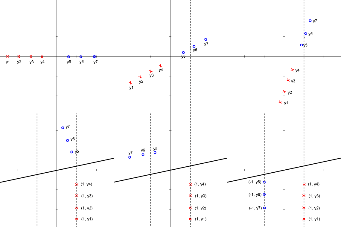
We attempt to find a linear projection (line that passes through the origin) s.t. the projected data can be "best" separated. The following animation shows how we can achieve the "best" separation between classes on the projected data by changing the projection plane $ \omega $.
- sorry, I did not realize that this image would change while I was working on [Lecture 11] I changed the name of the other image so whoever has the original animation can put it back**
Assume $ y_1,..., y_{d_1} $ belongs to Class 1 and $ y_{d_1+1} $,..., $ y_d $ belongs to Class 2.
Consider the sample mean of the projected data for each class
$ \tilde{m_1} = \frac{1}{d_1} \sum_{i=1}^{d_1} \pi(y_i) = \frac{1}{d_1}\sum_{i=1}^{d_1} \vec{w} \cdot y_i $, if $ ||\omega || =1 $
- Observation:** $ m1 = \vec{w} \frac{1}{d_1} \sum_{i=1}^{d_1} y_i $, which is the projection of the sample mean for Class 1.
Also, $ \tilde{m_2} = \frac{1}{d-d_1}\sum_{i=d_1+1}^{d} \vec{w} \cdot y_i = \vec{w} \cdot m_2 $ .
Consider the scatter projections:
$ \tilde{S_1}^2 = \sum_{i=1}^{d_1} (\vec{w} \cdot y_i - \tilde{m_1})^2 $
$ \tilde{S_2}^2 = \sum_{i=d_1+1}^{d} (\vec{w} \cdot y_i - \tilde{m_2})^2 $
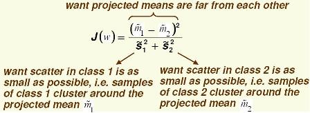
Define the following cost function, $ J(\vec{w}) = \frac{|\tilde{m1} - \tilde{m2}|^2}{\tilde{S_1}^2+ \tilde{S_2}^2} $ .
The above equation is the "[Fisher linear discriminant]".
- Observation:** Demanding $ ||\tilde{m_1} - \tilde{m_2}|| $ to be maximized would not do, since $ ||\tilde{m_1} - \tilde{m_2}|| = |\vec{w} \cdot m_1 - \vec{w} \cdot m_2 | = | \vec{w} \cdot (m_1 - m_2)| \rightarrow \infinity $
Need to fix $ || \omega || = 1 $ , resulting in a Constrained Optimization Problem.
By dividing by $ \tilde{S_1}^2 + \tilde{S_2}^2 $ we demand that $ \vec{w} \cdot (m_1 - m_2) $ be large in comparison with the scatter. This allows you to bypass the coordinate scale problem because $ J(\vec{w}) $ is independent of $ \omega $.
.. |eq2| image:: tex
- alt: tex: |\tilde{m_1} - \tilde{m_2}|^2 = | w(m_1 - m_2)|^2 = |w|^2 | \frac{w}{|w|}(m_1-m_2)|^2
.. |eq3| image:: tex
- alt: tex: \tilde{S_1}^2 = \sum (\vec{w}(y_i - m_1))^2 = |w|^2 \sum (\frac{w}{|W|} (y_i - m_1))^2
.. |eq4| image:: tex
- alt: tex: \tilde{S_2}^2 = \sum (\vec{w}(y_i - m_1))^2 = |w|^2 \sum (\frac{w}{|W|} (y_i - m_2))^2
$ |\tilde{m_1} - \tilde{m_2}|^2 = | w(m_1 - m_2)|^2 = |w|^2 | \frac{w}{|w|}(m_1-m_2)|^2 $
Similarly,
$ \tilde{S_1}^2 = \sum (\vec{w}(y_i - m_1))^2 = |w|^2 \sum (\frac{w}{|W|} (y_i - m_1))^2 $
and,
$ \tilde{S_2}^2 = \sum (\vec{w}(y_i - m_1))^2 = |w|^2 \sum (\frac{w}{|W|} (y_i - m_2))^2 $
and,
.. |eq5| image:: tex
- alt: tex: J(\vec{w}) = \frac{|m_1-m_2|^2}{S_1^2+S_2^2} =\frac{|w|^2 | \frac{w}{|w|}(m_1-m_2)|^2}{|w|^2(\sum (\frac{w}{|W|} (y_i - m_1))^2 + \sum (\frac{w}{|W|} (y_i - m_2))^2 )}
$ J(\vec{w}) = \frac{|m_1-m_2|^2}{S_1^2+S_2^2} =\frac{|w|^2 | \frac{w}{|w|}(m_1-m_2)|^2}{|w|^2(\sum (\frac{w}{|W|} (y_i - m_1))^2 + \sum (\frac{w}{|W|} (y_i - m_2))^2 )} $ is independent of $ ||\omega|| $.
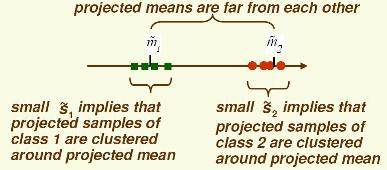
Importance of scatter:
If we find $ \omega $ which makes $ Jw $ large, we are guaranteed that the classes are well-separated.
We can write $ Jw $ using matrices:
$ J(\vec{w}) = \frac{\vec{w}^{\top}S_B \vec{w}}{\vec{w}^{\top}S_w \vec{w}} $, which is called the "[Generalized Rayleigh Quotient]".
([Lecture 11] begins here)
.. |fisher_1| image:: tex
- alt: tex: J(\vec{w})=\frac {{\vec{w}}^{T}{S}_{B}\vec{w}} {{\vec{w}}^{T}{S}_{W}\vec{w}}
.. |w_bar| image:: tex
- alt: tex: \vec{w}
.. |func_1| image:: tex
- alt: tex: \| \tilde{m_1}-\tilde{m_2} \|^2 = \| w(m_1-m_2) \|^2 = \| (m_1-m_2)^T w \|^2
.. |func_1_1| image:: tex
- alt: tex: =w^T (m_1-m_2)(m_1^T-m_2^T)w
.. |S_B| image:: tex
- alt: tex: (m_1-m_2)(m_1^T-m_2^T) =S_B
.. |func_2_1| image:: tex
- alt: tex: \tilde{s_1}^2 + \tilde{s_2}^2
.. |func_2_2| image:: tex
- alt: tex: \tilde{s_1}^2 =\displaystyle \sum_{\vec y \; in \; class} (w y_i- \tilde{m_i} )^2
.. |func_2_3| image:: tex
- alt: tex: =\displaystyle \sum_{\vec y \; in \; class}} w^T (y_i-m_i)(y_i^T-m_i^T)w
.. |func_2_4| image:: tex
- alt: tex: = w^T \displaystyle \sum_{\vec y \; in \; class}} (y_i-m_i)(y_i^T-m_i^T)w
.. |func_2_5| image:: tex
- alt: tex: \displaystyle \sum_{\vec y \; in \; class}} (y_i-m_i)(y_i^T-m_i^T) =S_w
Last time we considered $ J(\vec{w})=\frac {{\vec{w}}^{T}{S}_{B}\vec{w}} {{\vec{w}}^{T}{S}_{W}\vec{w}} $, explicit function of $ \vec{w} $
one can do this because
(numerator of J) = $ \| \tilde{m_1}-\tilde{m_2} \|^2 = \| w(m_1-m_2) \|^2 = \| (m_1-m_2)^T w \|^2 $
$ =w^T (m_1-m_2)(m_1^T-m_2^T)w $
where, |S_B| is 'between class scatter matrix'.
(denominator of J) = $ \tilde{s_1}^2 + \tilde{s_2}^2 $
$ \tilde{s_1}^2 =\displaystyle \sum_{\vec y \; in \; class} (w y_i- \tilde{m_i} )^2 $
$ =\displaystyle \sum_{\vec y \; in \; class}} w^T (y_i-m_i)(y_i^T-m_i^T)w $
$ w^T \displaystyle \sum_{\vec y \; in \; class}} (y_i-m_i)(y_i^T-m_i^T)w $
where, $ \displaystyle \sum_{\vec y \; in \; class}} (y_i-m_i)(y_i^T-m_i^T) =S_w $ is 'within class scattter matrix'.
From thanh.h.ha.1 Sat Feb 16 11:53:49 -0500 2008 From: thanh.h.ha.1 Date: Sat, 16 Feb 2008 11:53:49 -0500 Subject: the animation?? Message-ID: <20080216115349-0500@https://engineering.purdue.edu>
When the blue circles move down below the x axis, I think their cooridinates would change to(-1,-y5), (-1, -y6)...., not (-1,y5), (-1,y6)... as in the animation.


