(→Periodic Signals) |
(→Periodic Signals) |
||
| (4 intermediate revisions by the same user not shown) | |||
| Line 17: | Line 17: | ||
%%%Make second plot | %%%Make second plot | ||
| + | %Referenced code from Monil Goklani | ||
dt = pi/3.2; | dt = pi/3.2; | ||
time = 4*pi; | time = 4*pi; | ||
| Line 25: | Line 26: | ||
%Part 2 | %Part 2 | ||
| + | %referenced code | ||
%Function: x(t) = e^(t*j/6) | %Function: x(t) = e^(t*j/6) | ||
| Line 41: | Line 43: | ||
</pre> | </pre> | ||
| − | [[Image: | + | [[Image:HW2A1_ECE301Fall2008mboutin.jpg]] |
| − | [[Image: | + | [[Image:hw2Bdr_ECE301Fall2008mboutin.jpg]] |
Latest revision as of 18:00, 12 September 2008
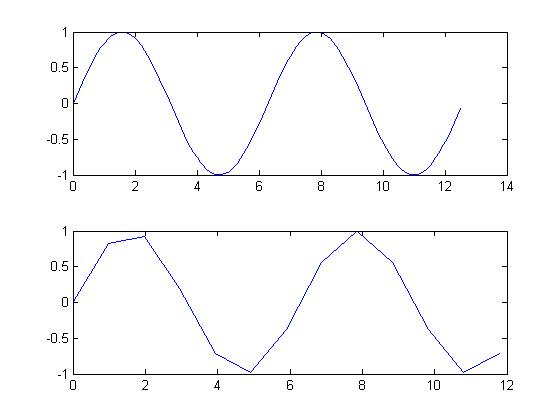
Periodic Signals
% Homework 2A Periodic Signals Revisited
%David Record
%September 3rd 2008

%Function f(x) = sin(x) -From Max Paganini's first homework
%%%Make first plot
dt = .1;
time = 4*pi;
t = [0:dt:time];
y = sin(t);
subplot(2,1,1);
plot(t,y);

%%%Make second plot
%Referenced code from Monil Goklani
dt = pi/3.2;
time = 4*pi;
t = [0:dt:time];
y = sin(t);
subplot(2,1,2);
plot(t,y);

%Part 2
%referenced code
%Function: x(t) = e^(t*j/6)

t=0.01:.01:1;
y=exp(t*j/6);
x=[]
for d=1:10
    x=[x,y];
end

t=[0.01:.01:10];
plot(t,x)


