(→Question 1) |
(→Question 2) |
||
| (7 intermediate revisions by the same user not shown) | |||
| Line 5: | Line 5: | ||
Recall that this signal is periodic if <math>T = {\omega_0\over2\pi}\,</math> is rational. | Recall that this signal is periodic if <math>T = {\omega_0\over2\pi}\,</math> is rational. | ||
| − | Say I choose the sampling | + | Say I choose the sampling period <math>T_s=.1\,</math> |
The output will be: | The output will be: | ||
| + | [[Image:Smooth_sin_ECE301Fall2008mboutin.jpg]] | ||
| + | But if I choose the sampling period to be <math>T_s=.7\,</math> | ||
| − | + | ||
| + | [[Image:Messed_sin_ECE301Fall2008mboutin.jpg]] | ||
| + | |||
| + | == Question 2 == | ||
| + | |||
| + | I'm including the code for this part because I found help using Tyler Houlihan's work. He apparently also received help from Wei Jian Chan's HW. I used Tyler's code as a base to recreate a periodic signal from: | ||
| + | |||
| + | <math>e^{-t}sin(t)\,</math> | ||
| + | |||
| + | Here's the code: | ||
| + | <pre> | ||
| + | %Creating 3 time vectors | ||
| + | t=[0:0.001:1.5;0:0.001:1.5;0:0.001:1.5]; | ||
| + | |||
| + | %setting the three variables, with their offsets | ||
| + | y =exp(-t(1,:)).*sin(t(1,:)); | ||
| + | y2=exp(-t(2,:)).*sin(t(2,:)); | ||
| + | y3=exp(-t(3,:)).*sin(t(3,:)); | ||
| + | |||
| + | %concatenating them, ie putting them after another | ||
| + | y4=[y,y2,y3]; | ||
| + | |||
| + | %making the new time axis for the whole thing | ||
| + | t=0:0.001:4.502; | ||
| + | |||
| + | %plotting | ||
| + | plot(t,y4); | ||
| + | </pre> | ||
| + | |||
| + | and the plot | ||
| + | |||
| + | |||
| + | [[Image: Periodic_ECE301Fall2008mboutin.jpg]] | ||
Latest revision as of 15:24, 11 September 2008
Question 1
I chose the signal $ x[n]=e^{j\pi n} \, $ which Jeff Kubascik posted on his HW1.
Recall that this signal is periodic if $ T = {\omega_0\over2\pi}\, $ is rational.
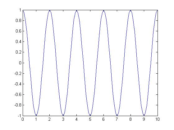
Say I choose the sampling period $ T_s=.1\, $
The output will be:
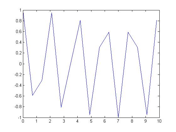
But if I choose the sampling period to be $ T_s=.7\, $
Question 2
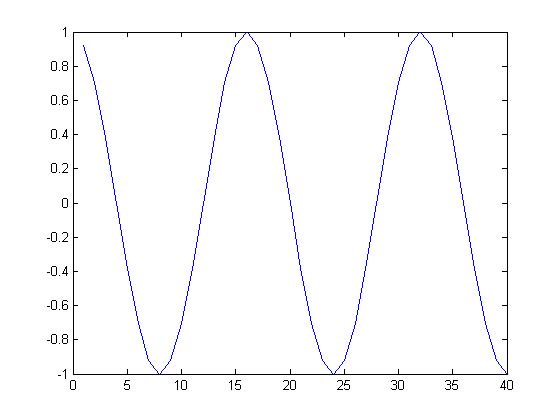
I'm including the code for this part because I found help using Tyler Houlihan's work. He apparently also received help from Wei Jian Chan's HW. I used Tyler's code as a base to recreate a periodic signal from:
$ e^{-t}sin(t)\, $
Here's the code:
%Creating 3 time vectors
t=[0:0.001:1.5;0:0.001:1.5;0:0.001:1.5];

%setting the three variables, with their offsets
y =exp(-t(1,:)).*sin(t(1,:));
y2=exp(-t(2,:)).*sin(t(2,:));
y3=exp(-t(3,:)).*sin(t(3,:));

%concatenating them, ie putting them after another
y4=[y,y2,y3];

%making the new time axis for the whole thing
t=0:0.001:4.502;

%plotting
plot(t,y4);
and the plot


