Back to Daniel's Honor Project
keywords: pca, eigenvalues, springs.
On Principal Component Analysis (PCA)
The other day, my friend E.E major friend, A.G., asked me if I knew what eigenvalues and eigenvectors were. I said no, because I didn't know what they were at the time. A.G. was working on his research project for detecting and characterizing movements of mice using Xbox kinect and wanted to understand and use principal component analysis (PCA) for image processing. He had not taken linear algebra yet; I was in the middle of taking the course. I promised him that I will tell him once I learn it in class.
Now, at the conclusion of my linear algebra course, I had acceptable understanding of linear algebra, elementary understanding of eigenvalues and eigenvectors, and, unfortunately, no idea of the utility of what I learned in the field of image processing. But, ideally, I now do have the background to understand PCA. I have spent a little time trying to understand what is achieved by applying PCA on a particular data. Although my interpretation of how PCA work is prone to errors, I hope the lack of sophistication in my language will render process of PCA understandable(without being entirely inaccurate).
I've relied heavily on the article by Jonathon Shlens's tutorial on PCA, inheriting his tutorial structure and examples. His article itself is a very readable and comprehensive one and can be accessed by clicking here.
Principal Component Analysis is a process of extracting useful information from a noisy data set. Complex data sets may hid significant relationship between variables, and the aim of PCA is to extricate those relevant information shrouded by unimportant data. So, really, its application is not limited to image processing.
What is a noisy, complex, clouded data?
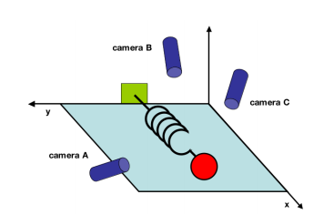
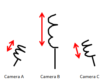
Suppose we have an oscillating ideal spring with a mass attached at its tip. This spring oscillates in one direction, namely in the x-direction, at a set frequency. We live in a three dimensional world, so we decide to set up three cameras in a rather random directions to collect the data on the motion of the spring.
This is not a brilliant idea. If we recall from our introductory physics course, the motion of the spring will always be in one-direction - the x-direction. So the entire dynamic of the spring system could be expressed with one variable, x. In lieu of three cameras recording the motion of the spring with respect to its axis, one camera positioned orthogonal to the motion of the spring would have sufficed.
In our hypothetical experiment, we record the x and y position of the spring every 0.1 second for 10 seconds, making 100 observations.
In the case of one camera positioned orthogonal to the spring's motion, one observation can be expressed as a matrix:
$ O_{n}=\left(\begin{array}{cccc}x_{n}\\y_{n}\end{array}\right) $
Since we would expect the value of x or y to be zero for all 100 observations (spring moves in only one direction), what we really have is data with one dimension. We can used the data to express the dynamic of the system with one variable, as we have expected.
What of the data collected via the dull positioning of the three cameras? Each camera will collect data in its own x,y direction. Each observation will assume the form:
$ O_{n}=\left(\begin{array}{cccc}x_{An}\\y_{An}\\x_{Bn}\\y_{Bn}\\x_{Cn}\\y_{Cn}\end{array}\right) $
This isn't such a friendly data, but it captures the dynamic of the spring's movement, albeit clumsily. Since we prefer to describe the dynamic of the spring system in simpler terms, how can use this data set to write the motion of spring in terms of just one variable, x? That is, how can re-express our data set so that the simple dynamics of the system is revealed?
We have a goal; we want to reduce the dimension of the data to present no redundancy. Also important is the strength, or signal, of our data. We define the two factors, redundancy and signal, with covariance and variance.
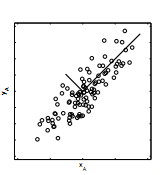
Suppose camera A records x and y position of the oscillating string, and we plot the data. Ideally, the points would form a single line, but in most experimental data will not exhibit ideal behavior due to noise. Therefore, if we assume that the dynamic in interest lies in the direction of greatest spread of the data, we come to correlate variance of the data with the strength of the signal- large variance means strong signal of data.
On the other hand, covariance of two variable measures the correlation between one variable to another. For example, if the value of correlation between x and y is large, value of x and y tend to increase or decrease in the same direction and thus is related somehow. In contrast, if the covariance between two variables is zero, then there is explicit relation between the two. We come to conclude that low covariance indicates low redundancy.
Then, we introduce the covariance matrix:
$ \sigma^2 = \left(\begin{array}{cccccc}\sigma^2_{x_A,x_A}&\sigma^2_{x_A,y_A}&\sigma^2_{x_A,x_B}&\sigma^2_{x_A,y_B}&\sigma^2_{x_A,x_C}&\sigma^2_{x_A,y_C}\\\sigma^2_{y_A,x_A}&\sigma^2_{y_A,y_A}&\sigma^2_{y_A,x_B}&\sigma^2_{y_A,y_B}&\sigma^2_{y_A,x_C}&\sigma^2_{y_A,y_C}\\:&:&:&:&:&:\\\sigma^2_{y_C,x_A}&\sigma^2_{y_C,y_A}&\sigma^2_{y_C,x_B}&\sigma^2_{y_C,y_B}&\sigma^2_{y_C,x_C}&\sigma^2_{y_C,y_C}\end{array}\right) $
Since we want to minimize the values of covariance and maximize the values of variances, ideally, we want entries along the diagonal to be nonzero and the entries outside the diagonal to be zero. In other words, we want to diagonalize the covariance matrix.


