The Greedy Method
Student project for MA375
Introduction
- We have completed data structures.
- We now are going to look at algorithm design methods.
- Often we are looking at optimization problems whose performance is exponential.
- For an optimization problem, we are given a set of constraints and an optimization
function.
o Solutions that satisfy the constraints are called feasible solutions.
o A feasible solution for which the optimization function has the best possible value
is called an optimal solution. - Cheapest lunch possible: Works by getting the cheapest meat, fruit, vegetable, etc.
- In a greedy method we attempt to construct an optimal solution in stages.
o At each stage we make a decision that appears to be the best (under some criterion) at the time.
o A decision made at one stage is not changed in a later stage, so each decision should assure feasibility. - Consider getting the best major: What is best now, may be worst later.
- Consider change making: Given a coin system and an amount to make change for, we
want minimal number of coins.
o A greedy criterion could be, at each stage increase the total amount of change
constructed as much as possible.
In other words, always pick the coin with the greatest value at every step.
o A greedy solution is optimal for some change systems. *Machine scheduling:
o Have a number of jobs to be done on a minimum number of machines. Each job has a start and end time.
o Order jobs by start time.
o If an old machine becomes available by the start time of the task to be assigned,
assign the task to this machine; if not assign it to a new machine. o This is an optimal solution. - Note that our Huffman tree algorithm is an example of a greedy algorithm: o Pick least weight trees to combine.
- Heuristic – we are not willing to take the time to get an optimal solution, but we can be satisfied with a “pretty good” solution.
0/1 Knapsack Problem - Problem description:
o Pack a knapsack with a capacity of c.
o From a list of n items, we must select the items that are to be packed in the knapsack.
o Each object i has a weight of wi and a profit of pi .
- In a feasible knapsack packing, the sum of the weights packed does not exceed the
knapsack capacity. - An optimal packing is a feasible one with maximum profit – ∑ p x subject to the constraints ∑wx ≤c and x ∈{0,1},1≤i≤n
o We are to find the values of xi where xi =1 if object i is packed into the knapsack and xi = 0 if object i is not packed. - Greedy strategies for this problem:
o From the remaining objects, select the object with maximum profit that fits into
the knapsack.
o From the remaining objects, select the one that has minimum weight and also fits
into the knapsack.
o From the remaining objects, select the one with maximum pi / wi that fits into the
knapsack.
- Consideraknapsackinstancewheren=4, w=[2,4,6,7], p=[6,10,12,13],and c=11.
o Look at the above three strategies. - None of the above algorithms can guarantee the optimal solution.
o This is not surprising since this problem is a NP-hard problem. - Of the above three algorithms, the third one is probably the best heuristic.
Topological Ordering - Greedy criteria – for the unnumbered nodes, assign a number to a node for which all predecessors have been numbered.
• Algorithm – Initially, for each node with predecessor count of zero, put it in a container (stack, queue, anything will do).
1. Remove a node with predecessor count of zero from the container, number it, then list it.
2. For each successor, decrement its predecessor count.
3. If a successor now has a predecessor count of zero, add it to the container. - Complexity – assume an adjacency list.
1. Find predecessor count. Ο(e) , where e is number of edges.
2. List node – for each successor, update predecessor count. Ο(e + n) , since if have
lots of nodes with no predecessors, n could be more than e.
Matchings and Coverings in a Graph
- Matching – a set of edges, no two of which have a vertex in common.
- A perfect match is one in which all vertices are matched.
- A maximum matching is matching that cannot be extended by the addition of an edge.
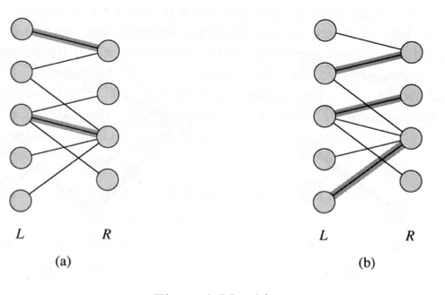
- For an example see Figure 1.
Figure 1 Matching
- Many problems that seem unrelated to matching can be formulated this way.
- Edge covering – find minimum number of edges (not necessarily independent) to cover
(touch) all vertices. - Stable marriage problem – we want to find a matching such that there exists no situation
in which two individuals would rather be matched with each other than the people they are currently matched with.
Bipartite Cover - Bipartite graph – (two parts) two independent sets of vertices such that all edges are between elements of different sets.
- Complete bipartite – every vertex of one set is adjacent to every vertex of second set.
- Examples of bipartite graphs:
o Would-work-for graph in which one set of nodes is jobs and another set is employees.
o Want to marry (in Utah) where the node sets are men and women. - Cover – a subset A' of the set A is said to cover the set B iff every vertex in B is connected
to at least one vertex of A'.
o Size of the cover – the number of vertices in A'.
o Minimum cover – there is no smaller subset of A that covers B. - Bipartite cover – given two types of nodes X and Y, X' is a node cover if X' is a subset of X such that every node in Y is connected to a node in X' via an edge. We want the cover of the minimum size.
- A covering for Figure 2 is {1, 2, 3, 17}.
• Show the minimum cover for the bipartite graph shown in Figure 2.
o The cover is {1, 16, 17}.
Figure 2 Bipartite Graph
• Examples:
o Suppose you have a set of interpreters and a set of languages that need to be
interpreted. Edges represent “can interpret.” We want to find the minimal
number of interpreters to hire so that you can interpret all languages.
o Set of people and a set of categories (male, Asian, CS major, single, ...). We want
to form a committee with representation from all groups.
• Set cover – given a collection of subsets, find a minimum number of subsets such that
their union is the universe.
o Can you see how to map this problem to the bipartite cover problem?
Nodes for each subset. Nodes for each element. Edges represent “contains.”
• This ability to map one problem into another is key to using knowledge of “algorithms community.” This is likely the reason why I always try to find similarities between things that seem different (e.g., cleaning up for company).
• NP-hard – no one has developed a polynomial time algorithm. o Also called intractable or exponential.
o We use greedy algorithms to approximate.
• Greedy criterion – Select the vertex of A that covers the largest number of uncovered vertices of B. Also keep a Boolean array that tells whether each node is covered or not.
o This idea could be implemented via a max tournament tree of “willCover” – take the biggest.
Shortest Paths
• Given a digraph with each edge in the graph having a nonnegative cost (or length).
• Try to find the shortest paths (in a digraph) from a node to all other nodes.
• Greedy criterion – From the vertices to which the shortest path has not been generated,
select one that results in the least path length (the smallest one).
• Have a reached set of nodes and an unreached set of nodes.
1. Initially, only the start node is reached.
2. Use a min priority queue to store the total path lengths of each of the reached nodes to its successors.
3. While priority queue is not empty
Pick the shortest total length node.
• If it has already been reached, discard.
• Else count it as reached.
Enqueue the total path lengths of each of the reached nodes to its
successors.
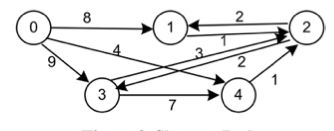
• For example, consider the digraph Figure 3 in and calculate the shortest path.

Figure 3 Shortest Path
Minimal Spanning Trees
• Problem – select a subset of the edges such that a spanning tree is formed and the weight of the edges is minimal.
• Example – need to connect all sites to sewer system - want to minimize the amount of pipe.
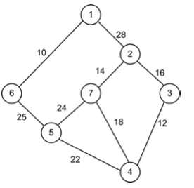
• Consider the spanning tree shown in Figure 4.
• Prim’s algorithm
o Greedy criterion – From the remaining edges, select a least-cost edge whose
addition to the set of selected edges forms a tree. Tree – set of vertices already in MST
Succ – set of vertices not in Tree but in Succ[Tree] Place any vertex (to serve as root) in MST.
The Greedy Method
Page 5
1. Find the smallest edge that connects Tree with Succ
2. Add the edge to the MST and update Tree and Succ
• Uses a greedy method – obtain a globally optimal solution by means of a locally optimal
solution.
• Using Figure 4 and Prim’s algorithm, we add the edges in the following order: (1,6),
(6,5), (5,4), (4,3), (3,2), and (2, 7).
• How do we find smallest edge? (sort or priority queue)
• Kruskal’s algorithm
o Greedy criterion – From the remaining edges, select a least-cost edge that does not result in a cycle when added to the set of already selected edges.
Let each vertex be a separate component.
1. Examine each edge in increasing order of cost.
2. If edge connects vertices in same component, discard it. Otherwise, add edge to
MST. Update components.
• Using Figure 4 and Kruskal’s algorithm, we add the edges in the following order: (1,6),
(3,4), (2,7), (2,3), (4,5), and (5,6).
• How do we find smallest edge? (sort or priority queue)
More Traversals of a Graph or Digraph
• Tour – visit each vertex in a graph exactly once and finish at the vertex started from.
• Eulerian tour – find a path/tour through the graph such that every edge is visited
exactly once. (Easy – check nodal degree; if all are even, it is possible.)
• Hamiltonian tour – find a path through the graph such that every vertex is visited
exactly once. (NP complete)
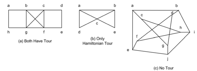
• See Figure 5 for different tours.


