Sampling rate conversion: an intuitive view
Background:
In signal processing, sampling is the act of converting a continuous-time (CT) signal into a discrete-time (DT) one. Although it may be easier to mathematically process a CT signal directly, this is not possible in reality since storing a real-world signal would require an infinite amount of memory. Consequently, all signals are sampled before being processed by a computer system. Sampling is performed at a certain rate limited by hardware known as the sampling rate/frequency (samples per second, or Hz), or with a certain time between samples known as the sampling period (seconds). It should be noted that these terms are reciprocals of each other. That is,
$ f_s = \frac{1}{T_s} $
The connection between these two terms means that when we reduce the sampling rate, we increase the sampling period and vice versa. Therefore, reducing the sampling rate increases the length of time between consecutive measurements.
With this information, we can express the sampling of a CT signal $ x(t) $ in terms of its sampling period T:
$ x(t) → $ sampling with period T $ → x(nT) = x[n] $
The result of this expression, $ x[n] $, is a discrete time signal where each value is taken from $ x(t) $ at an integer multiple of the sampling period T. Therefore, the CT signal $ x(nT) $ is equivalent to the DT signal $ x[n] $, where $ n $ is an integer and indexes the DT signal.
If a DT signal is created by sampling a CT signal faster than a certain rate known as the Nyquist rate, the original CT signal can be perfectly reconstructed from the DT sampling. The Nyquist rate, $ f_0 $, is defined as:
$ f_0 = 2f_{max} $, where $ f_{max} $ is the greatest frequency in the signal of interest, $ x(t) $.
If the sampling rate of a signal is not greater than $ f_0 $, the sampled signal will exhibit aliasing, which results when two distinct frequency bands overlap in the Fourier domain. In other words, aliasing occurs when the original signal’s frequency profile is altered after sampling. In this case, the CT signal cannot be reconstructed from the DT sampling without error.
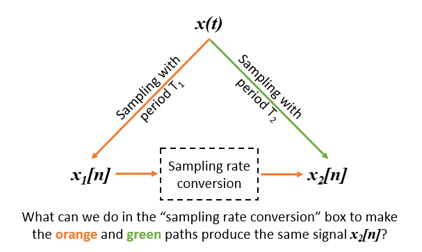
For the purpose of this report, we will assume that we have measured a band-limited, real-world signal $ x(t) $ with maximum frequency $ f_{max} $ (in Hz). During measurement, the CT signal is sampled with sampling rate $ f_1 = \frac{1}{T_1} $ to produce a DT signal $ x(nT_1) = x_1[n] $. Note that the original time-domain signal is not accessible because it cannot be stored by a computer. The question is: can we convert the sampled signal $ x_1[n] $ to a different signal $ x_2[n] $ with sampling rate $ T_2 $ that is equivalent to a signal obtained by directly sampling $ x(t) $ with sampling period $ T_2 $? See below for an illustration of this question:
As we will see, it is indeed possible to obtain $ x_2[n] $ from $ x_1[n] $ by various means--downsampling, decimation, upsampling, and interpolation--collectively known as sampling rate conversion.
Downsampling:
We will begin by providing a motivating example for downsampling. Let’s say that a scientist aboard the International Space Station (ISS) would like to communicate with the engineers at Mission Control. The scientist’s voice has a maximum frequency $ f_{max} = 1,000 $ Hz, and the high-end analog-to-digital converters in his communication radio sample his speech well above the Nyquist rate at $ f_s = 10,000 $ Hz. However, a signal sampled this quickly contains a large number of data points, which will greatly increase the transmit power required to send the signal back to Earth. Due to limited power availability aboard the ISS, the scientist would like to keep all communications as low-power as possible. What can the scientist do to reduce his power consumption?
To reduce the required transmit power, the sampling rate of the speech signal must be reduced, or downsampled. Downsampling allows us to extract a second signal $ x_2[n] $ with sampling period $ T_2 $ from another signal $ x_1[n] $ with lower sampling period $ T_1 $. That is, downsampling requires $ T_2 > T_1 $, where $ T_2 $ is proportional to $ T_1 $ by a factor $ D $, which is an integer greater than 1. From this, we establish the following relationship:
$ T_2 = DT_1 $
or equivalently
$ T_1 = \frac{T_2}{D} $ (1)
The second equation may be useful in the future to help distinguish downsampling from upsampling, in that $ T_1 $ and $ T_2 $ appear in order left-to-right, and the factor $ D $ appears below (down from) $ T_2 $. Overall, downsampling creates a new signal $ x_2[n] $ that consists of only every $ D^{th} $ sample of $ x_1[n] $.
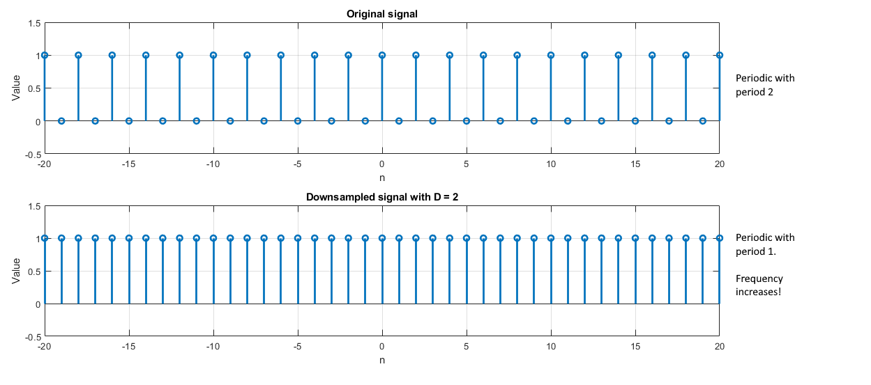
In the time domain, downsampling effectively removes all data between each $ D^{th} $ sample. In the frequency domain, this process increases the signal’s maximum frequency (and therefore its bandwidth) and decreases its amplitude, both by a factor $ D $. Why does this happen? Let’s take a look at an example.
Let $ x_{10000}[n] $ be the scientist’s speech signal sampled at 10,000 Hz. Note that 10,000 Hz is the sampling frequency, so the sampling period, $ T_s = \frac{1}{f_s} $, is 1/10000 seconds (0.1 ms). To save transmission power, he would like to downsample the signal by a factor of $ D = 4 $ to reduce the sampling rate $ f_s $ to 2,500 Hz ($ T_s = 1/2500 $ seconds, 0.4 ms). From the connection between sampling rate and sampling period, it may seem like this increase in time between samples will decrease the maximum frequency of the original signal since samples are being taken less often (less frequently). However, it is important to note that this is not the case. Instead, the maximum frequency of the downsampled signal actually increases because samples of that frequency are moved closer together when data between them is removed. See the illustration below:
This explains the bandwidth increase seen after downsampling. The amplitude decrease is related to the Fourier transform formula.
Because downsampling increases the bandwidth of the original signal, one must be careful to prevent aliasing. To ensure that no aliasing occurs when downsampling, $ x_2[n] $ must satisfy the Nyquist criterion. It can be shown that if $ x_2[n] $ has a lower sampling rate than $ x_1[n] $, if $ x_2[n] $ satisfies Nyquist, then $ x_1[n] $ will also. To meet this condition mathematically, we require:
$ f_{max} < \frac{1}{2T_2} $ (2)
or equivalently
$ f_{max} < \frac{1}{2DT_1} $, since $ T_2 = DT_1 $
If we look at these requirements in terms of radians/sec which is commonly used when expressing the discrete-time Fourier transform, we get:
$ 2𝜋T_1f_{max} < \frac{𝜋}{D} $ (3)
or equivalently
$ 2𝜋T_2f_{max} < 𝜋 $, since $ T_2 = DT_1 $
This conversion comes from the fact that $ w = 2𝜋f $ in continuous time. However, a sampled signal introduces an extra factor $ T $, which is the sampling period of the signal. From this, we define the discrete time frequency $ w = 2𝜋fT $.
Finally, one should note that downsampling a signal with original sampling period $ T_0 $ by a factor $ D $ is equivalent to resampling that signal with sampling period $ T_1 = DT_0 $. In terms of the initial sampled signal $ x_1[n] $ and its downsampled version $ x_2[n] $, we have:
$ x_2[n] = x_1[nD] $
Decimation:
Sometimes it is not possible to prevent aliasing in a sampled signal. We will provide an example of this by changing the scenario given above. Let’s say that it is the birthday of one of the engineers at Mission Control and the scientists aboard the ISS want to send them the “Happy Birthday” song which has $ f_{max} = 3,000 $ Hz. As before, the scientists would like to downsample the song by a factor of $ D = 4 $ before transmission to conserve power, but this will cause aliasing since $ f_{max} $ will increase to 12,000 Hz after downsampling. How can the song be sent without introducing aliasing?
In cases where the sampling rate is not sufficient to prevent aliasing after downsampling, decimation can be used instead. This technique will remove high frequency content from the original signal by first passing it through a low pass filter to ensure the final downsampled signal satisfies the Nyquist criterion. See the illustration below:
$ x_1[n] $ → Low pass filter with cutoff $ \frac{𝜋}{D} $ and gain 1 → Downsample by factor $ D → x_2[n] $
This technique is used to band-limit $ x_1[n] $ to $ \frac{𝜋}{D} $ before downsampling by a factor of $ D $ which increases the frequency range back to [-𝜋, 𝜋]. This process guarantees that no aliasing occurs because the DTFT of a signal with bandwidth 2𝜋 (and period 2𝜋, by the definition of the DTFT) will never overlap itself. However, some high frequency content from the original signal is inevitably lost.
For our example the original sampled signal $ x_1[n] $ sampled at $ T_1 = 10,000 $ Hz must first be low pass filtered with a cutoff frequency of $ \frac{𝜋}{D} = \frac{𝜋}{4} $ to remove the frequency content that will cause aliasing when its bandwidth is increased by a factor of 4. Downsampling by a factor of 4 will then cause the bandwidth to fill [-𝜋, 𝜋]. The result will be $ x_2[n] $, sampled at 2,500 Hz. Although some high frequency content was lost, the resulting signal does not show aliasing in the frequency domain, which would have occurred if the low pass filter was not applied.
It is important to note that downsampling and decimation produce equivalent results if the original signal $ x_1[n] $ satisfies the Nyquist condition for the sampling period $ T_2 $ of the downsampled signal $ x_2[n] $. In other words, if no aliasing will occur after downsampling (equations (2) and (3) are satisfied), the low pass filter used in decimation will have no effect, and both processes will produce the same result. In the example where the scientist only sought to transmit his voice, both downsampling and decimation would have produced the same result since $ f_{max} $ after downsampling would be 4 * 1,000 Hz = 4,000 Hz. Since $ f_s = 10,000 $ Hz $ < 2f_{max, 2} = 8,000 $ Hz, the Nyquist criterion is satisfied for $ T_2 = 1 / 4,000 $.
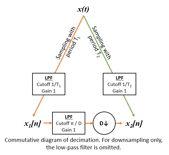
Below is a summary of downsampling and decimation in pictorial form:
Note the low pass filters used when sampling $ x(t) $ with period $ T_1 $ and $ T_2 $. We use these filters because we have specified that $ f_{max} > \frac{1}{2T_1} $, so aliasing is guaranteed to occur when sampling with $ T_1 $. If aliasing will occur with smaller sampling period $ T_1 $, it is also guaranteed to occur with larger sampling period $ T_2 $, hence the cutoff frequency of $ \frac{1}{2T_2} $ for $ x_2[n] $. These filters ensure that no aliasing occurs during the initial sampling of $ x(t) $ to create $ x_1[n] $ and $ x_2[n] $.
Upsampling:
There are some instances in which the sampling rate of a given signal is lower than we would like it to be for processing. To demonstrate this, we will continue our previous scenario by imagining that the engineer’s radio at Mission Control has a fixed playback rate of 10,000 Hz. If he tries to play the signals sent by the scientist in the ISS back at this rate, they will be played 4x too fast. To solve this problem and to play back the audio at the proper speed, the engineer must upsample the signal by a factor of 4 to bring its sampling rate back to 10,000 Hz.
In contrast to downsampling and decimation, upsampling allows us to extract a second signal $ x_2[n] $ with sampling period $ T_2 $ from another signal $ x_1[n] $ with higher sampling period $ T_1 $. In other words, upsampling requires $ T_1 > T_2 $, where $ T_1 $ is proportional to $ T_2 $ by a factor $ D $, which is an integer greater than 1. In the time domain, $ x(nT_1) $ is sampled less often than $ x(nT_2) $. With this, we can establish the following relationship:
$ T_1 = DT_2 $
If we compare the above equation to equation (1), we can see a convenient pattern in upsampling versus downsampling. In the upsampling formula above, $ T_1 $ and $ T_2 $ appear in order left-to-right, and the factor $ D $ appears in the numerator (up) with $ T_2 $. Overall, upsampling creates a new signal $ x_2[n] $ by placing $ D - 1 $ zeros between every sample of a given signal $ x_1[n] $. This process is also known as zero-padding. Mathematically, we can represent the relationship between $ x_1[n] $ and $ x_2[n] $ as:
$ x_2[n] = \begin{cases} x_1[\frac{n}{D}] & \text{if n / D is integer} \\ 0 & \text{otherwise} \end{cases} $
In the time domain, zero-padding causes the samples of $ x[n] $ to occur less often, thereby decreasing the frequency content of the signal. In the frequency domain, this compresses the frequency axis by a factor $ D $ so that multiple copies of the original signal may appear in the range [-𝜋, 𝜋]. The new signal is now periodic with period $ \frac{2𝜋}{D} $. This rescaling also increases the amplitude of the upsampled signal’s frequency profile by a factor $ D $ by the definition of the Fourier transform.
Similar to the fact that downsampling is not necessarily the best way to decrease the sampling rate of a signal, upsampling is not necessarily the best way to increase the sampling rate of a signal. When the signal’s frequency content is scaled down by a factor $ D $, more copies of the signal may appear in the interval [-𝜋, 𝜋]. These extra copies contribute to aliasing when the signal is transformed back to the time domain. To fix this, the upsampling equivalent of decimation known as interpolation can be used.
Interpolation:
Aliasing introduced by upsampling can be prevented by low pass filtering the upsampled signal with a cutoff frequency of $ \frac{𝜋}{D} $ and gain $ D $. This low pass filter eliminates the frequency copies not centered directly around $ w = 0 $ in the frequency domain. See the diagram below:
$ x_1[n] $ → upsample by factor $ D $ → low pass filter with cutoff $ \frac{𝜋}{D} $ and gain $ D → x_2[n] $
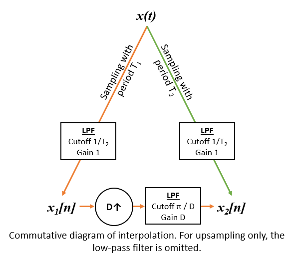
The low-pass filter ensures that only the center frequency copy remains in the interval [-𝜋, 𝜋] and eliminates aliasing when the inverse Fourier transform is taken. See the diagram below for an overview of upsampling/interpolation:
Summary:
In summary, downsampling, decimation, upsampling, and interpolation can all be used to convert one sampling rate to another. In some cases, care must be taken to prevent aliasing. These methods allow one to convert a given sampled signal into a second signal sampled at a different rate, which can be useful in many situations.


