Discriminant Functions For The Normal Density - Part 2
Continuing from where we left of in Part 1, in a problem with feature vector y and state of nature variable w, we can represent the discriminant function as:
$ g_i(\mathbf{x}) = - \frac{1}{2} \left (\mathbf{x} - \boldsymbol{\mu}_i \right)^t\boldsymbol{\Sigma}_i^{-1} \left (\mathbf{x} - \boldsymbol{\mu}_i \right) - \frac{d}{2} \ln 2\pi - \frac{1}{2} \ln |\boldsymbol{\Sigma}_i| + \ln P(w_i) $
we will now look at the multiple cases for a multivariate normal distribution.
Case 1: Σi = σ2I
This is the simplest case and it occurs when the features are statistically independent and each feature has the same variance, σ2. Here, the covariance matrix is diagonal since its simply σ2 times the identity matrix I. This means that each sample falls into equal sized clusters that are centered about their respective mean vectors. The computation of the determinant and the inverse |Σi| = σ2d and Σi-1 = (1/σ2)I. Because both |Σi| and the (d/2) ln 2π term in the equation above are independent of i, we can ignore them and thus we obtain this simplified discriminant function:
$ g_i(\mathbf{x}) = - \frac{||\mathbf{x} - \boldsymbol{\mu}_i||^2 }{2\boldsymbol{\sigma}^{2}} + \ln P(w_i) $
where ||.|| denotes the Euclidean norm, that is,
$ ||\mathbf{x} - \boldsymbol{\mu}_i||^2 = \left (\mathbf{x} - \boldsymbol{\mu}_i \right)^t (\mathbf{x} - \boldsymbol{\mu}_i) $
If the prior probabilities are not equal, then the discriminant function shows that the squared distance ||x - μ||2 must be normalized by the variance σ2 and offset by adding ln P(wi); therefore if x is equally near two different mean vectors, the optimal decision will favor the priori more likely. Expansion of the quadratic form (x - μi)t(x - μi) yields :
$ g_i(\mathbf{x}) = -\frac{1}{2\boldsymbol{\sigma}^{2}}[\mathbf{x}^t\mathbf{x} - 2\boldsymbol{\mu}_i^t\mathbf{x} + \boldsymbol{\mu}_i^t\boldsymbol{\mu}_i] + \ln P(w_i) $
which looks like a quadratic function of x. However, the quadratic term xtx is the same for all i, meaning it can be ignored since it just an additive constant, thereby we obtain the equivalent discriminant function:
$ g_i(\mathbf{x}) = \mathbf{w}_i^t\mathbf{x} + w_{i0} $
where
$ \mathbf{w}_i = \frac{1}{\boldsymbol{\sigma}^{2}}\boldsymbol{\mu}_i $
and
$ w_{i0} = -\frac{1}{2\boldsymbol{\sigma}^{2}}\boldsymbol{\mu}_i^t\boldsymbol{\mu}_i + \ln P(w_i) $
wi0 is the threshold or bias for the ith category.
A classifier that uses linear discriminants is called a linear machine. For a linear machine, the decision surfaces for a linear machine are just pieces of hyperplanes defined by the linear equations gi(x) = gj(x) for the two categories with the highest posterior probabilities. In this situation, the equation can be written as
$ \mathbf{w}^t(\mathbf{x} - \mathbf{x}_0) = 0 $
where
$ \mathbf{w} = \boldsymbol{\mu}_i - \boldsymbol{\mu}_j $
and
$ \mathbf{x}_0 = \frac{1}{2}(\boldsymbol{\mu}_i + \boldsymbol{\mu}_j) - \frac{\boldsymbol{\sigma}^{2}}{||\boldsymbol{\mu}_i - \boldsymbol{\mu}_j||^2}\ln\frac{P(w_i)}{P(w_j)}(\boldsymbol{\mu}_i - \boldsymbol{\mu}_j) $
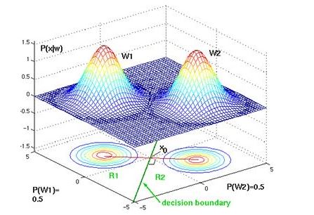
The equations define a hyperplane through the point x0 and orthogonal to the vector w. Because w = μi - μj, the hyperplane separating Ri and Rj is orthogonal to the line linking the means. if P(wi) = P(wj), the point x0 is halfway between the means and the hyperplane is the perpendicular bisector of the line between the means in fig1 below. If P(wi) ≠ P(wj), the point x0 shifts away from the more likely mean.
Case 2: Σi = Σ
Another case occurs when the covariance matrices for all the classes are identical. It corresponds to a situation where the samples fall into hyperellipsoidal clusters of equal size and shape, with the cluster of the ith class being centered around the mean vector μi. Both |Σi| and the (d/2) ln 2π terms can also be ignored as done in the first step because they are independent of i. This leads to the simplified discriminant function:
$ g_i(\mathbf{x}) = - \frac{1}{2} \left (\mathbf{x} - \boldsymbol{\mu}_i \right)^t\boldsymbol{\Sigma}_i^{-1} \left (\mathbf{x} - \boldsymbol{\mu}_i \right) + \ln P(w_i) $
If the prior probabilities P(wi) are equal for all classes, then the ln P(wi) term can be ignored, however if they are unequal then the decision will be biased in favor of the more likely priori. Expansion of the quadratic form ('x - μi)tΣ-1(x - μi) results in a sum involving the term xtΣ-1'x which is independent of i. After this term is dropped, we get the resulting linear discriminant function:
$ g_i(\mathbf{x}) = \mathbf{w}_i^t\mathbf{x} + w_{i0} $
where
$ \mathbf{w}_i = \boldsymbol{\Sigma}^{-1}\boldsymbol{\mu}_i $
and
$ w_{i0} = -\frac{1}{2}\boldsymbol{\mu}_i^t\boldsymbol{\Sigma}^{-1}\boldsymbol{\mu}_i + \ln P(w_i) $
Because the discriminants are linear, the resulting decision boundaries are again hyperplanes. If Ri and Rj are very close, the boundary between them has the equation:
$ \mathbf{w}^t(\mathbf{x} - \mathbf{x}_0) = 0 $
where
$ \mathbf{w} = \boldsymbol{\Sigma}^{-1}(\boldsymbol{\mu}_i - \boldsymbol{\mu}_j) $
and
$ \mathbf{x}_0 = \frac{1}{2}(\boldsymbol{\mu}_i + \boldsymbol{\mu}_j) - \frac{\ln[P(w_i)/P(w_j)]}{(\boldsymbol{\mu}_i - \boldsymbol{\mu}_j)^t\boldsymbol{\Sigma}^{-1}(\boldsymbol{\mu}_i - \boldsymbol{\mu}_j)}(\boldsymbol{\mu}_i - \boldsymbol{\mu}_j) $
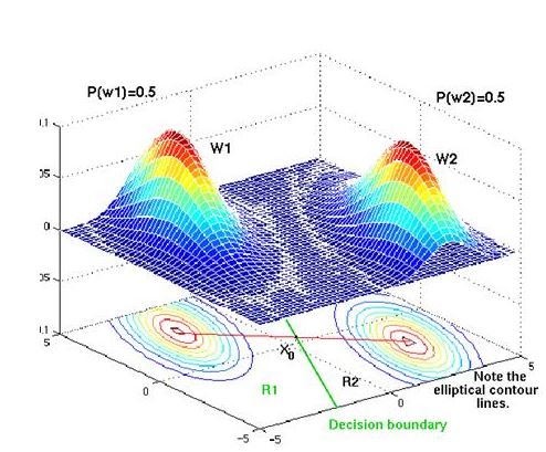
Because w = σ-1(μi - μj) is generally not in the direction of μi - μj, the hyperplane separating Ri and Rj is generally not orthogonal to the line between the means. If the prior probabilities are equal, it intersects the line at point x0, and then x0 is halfway between the means. If the prior probabilities are not equal, the boundary hyperplane is shifted away from the more likely mean. Figure 2 below shows what the boundary decision looks like for this case
Case 3: Σi = arbitrary
In the general multivariate Gaussian case where the covariance matrices are different for each class, the only term that can be dropped from the initial discriminant function is the (d/2) ln 2π term. The resulting discriminant term is;
$ g_i(\mathbf{x}) = \mathbf{x}^t\mathbf{W}_i\mathbf{x} + \mathbf{w}_i^t\mathbf{x} + w_{i0} $
where
$ \mathbf{W}_i= -\frac{1}{2}\boldsymbol{\Sigma}_i^{-1} $
$ \mathbf{w}_i= \boldsymbol{\Sigma}_i^{-1}\boldsymbol{\mu}_i $
and
$ w_{i0} = -\frac{1}{2}\boldsymbol{\mu}_i^t\boldsymbol{\Sigma}_i^{-1}\boldsymbol{\mu}_i - \frac{1}{2}\ln|\boldsymbol{\Sigma}_i|+ \ln P(w_i) $
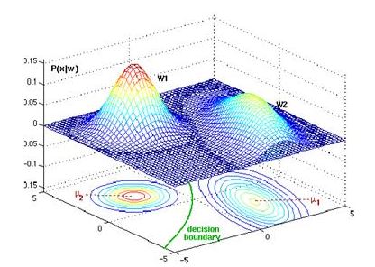
This leads to hyperquadric decision boundaries as seen in the figure below.
EXAMPLE
Given the set of data below of a distribution with two classes w1 and w2 both with prior probablility of 0.5, find the discriminant functions and decision boundary.
| Sample | w1 | w2 |
| 1 | -5.01 | -0.91 |
| 2 | -5.43 | 1.30 |
| 3 | 1.08 | -7.75 |
| 4 | 0.86 | -5.47 |
| 5 | -2.67 | 6.14 |
| 6 | 4.94 | 3.60 |
| 7 | -2.51 | 5.37 |
| 8 | -2.25 | 7.18 |
| 9 | 5.56 | -7.39 |
| 10 | 1.03 | -7.50 |
From the data given above we know to use the equations from case 1 since all points in each class have the same variance, therefore the means are:
$ \boldsymbol{\mu}_1 = \sum_{k=1}^{10}\mathbf{x}_1 = -0.44 $
$ \boldsymbol{\mu}_2 = \sum_{k=1}^{10}\mathbf{x}_2 = -0.543 $
and the variances are
$ \boldsymbol{\sigma}_1^2 = \sum_{k=1}^{10}\mathbf{x}_1 - \boldsymbol{\mu}_1 = 31.34 $
$ \boldsymbol{\sigma}_2^2 = \sum_{k=1}^{10}\mathbf{x}_2 - \boldsymbol{\mu}_2 = 52.62 $
The discriminant functions are then
$ g_1 = \frac{-0.44}{31.34} - \frac{-0.44^2}{2*31.34} +\ln(0.5) = -0.710 $
$ g_2 = \frac{-0.543}{52.62} - \frac{-0.543^2}{2*52.62} +\ln(0.5) = -0.706 $
and the decision boundary x0 is going to be halfway between the means at 0.492 because they have the same prior probability.


