Before logistic model
After the discussion of the background information related to population projection, we will take a close look at one of the simplest yet famous mathematical models for the population projection: the logistic model. But we need to understand the exponential model first, since the logistic model is developed based on the exponential model.
The significance of the exponential model is that it reflects a geometric population growth, which will be inherited by the logistic model. The geometric population growth is first proposed in 1798 by Thomas Robert Malthus in his An Essay on the Principle of Population, as It Affects the Future Improvement of Society, With Remarks on the Speculations of Mr. Godwin, Mr. Condorcet and Other Writers. He stated that “Population, when unchecked, increased in a geometric ratio.” He also believed that “Subsistence increases only in an arithmetical ratio.” Therefore, Malthus predicted that human society will eventually end up with famine. This publication had tremendous influences on studies of population and it allowed Malthus to become the founder of the exponential population model.
The exponential population model has the following form:$ P(t)=P_0e^rt. $
Where
- $ P_0=P(0) $ is the initial population size,
- $ r $is the population growth rate, also known as Malthusian Parameter,
- $ t $ is the time.
This model also has a differential form:$ \frac{dP}{dt}=rP $
The following calculation will lead to lead to the model above
As $ P(T) $ and $ P(0) $ are all positive, the solution is:$ P(t)=P_0e^{rt} $
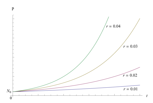
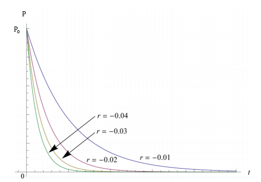
The population growth rate is the deterministic factor in this model. Following are graphs of the population with different growth rate:
Figure 4.1. The Exponential with positive population growth rate. Adapted from “Mathematical Models in Population Dynamics,” by Alexander Salisbury.
Figure 4.2. The Exponential with positive population growth rate. Adapted from “Mathematical Models in Population Dynamics,” by Alexander Salisbury.
The x-axis is representing the time, and the y-axis is the population. When r is positive, increase of r leads to the dramatic growth in population size. Meanwhile, with negative r, the decrease of r contributes to the smoothness of population decay. This growth rate is also essential in the logistic model, which will be discussed in the later sessions.
Although Malthus’ idea is influential, the model itself is not very practical. The model had following assumptions: “the population is homogeneous (i.e., all members are identical); the population inhabits a uniform and unvarying environment; an infinite supply of nutrients is available; there are no spatial limitations, and growth is density-independent.” In reality, those assumptions can easily be broken in the long term. Hence, more realistic models are required.


