From Bayes' Theorem to Pattern Recognition via Bayes' Rule
Partly based on the ECE662 Spring 2014 lecture material of Prof. Mireille Boutin.
Contents
What will you learn from this slecture?
- Bayes' Theorem: definition, derivation, and intuition.
- The classification problem setting in pattern recognition.
- Bayes' Rule: derivation, importance and, the difference between Bayes' rule and Bayes' theorem.
Historical Note
Bayes' Theorem takes its name from the mathematician Thomas Bayes. For an accurate and detailed information about Bayes, you might want to read his biography by Prof. D.R. Bellhouse [1]
Prerequisite
This tutorial assumes familiarity with the following--
- The axioms of probability
- Definition of conditional probability
Bayes' Theorem
Let us revisit conditional probability through an example and then gradually move onto Bayes' theorem.
Example
Problem: In Spring 2014, in the Computer Science (CS) Department of Purdue University, 200 students registered for the course CS180 (Problem Solving and Object Oriented Programming). 30% of the registered students are CS majors and the rest are non-majors. From the student registration data we observe that 80% of the CS majors are males, where as only 40% of non-majors are males. Find the following:
- The probability that a randomly selected student is a CS major.
- The probability that the selected student is a CS major and a male.
- The probability that the selected student is a male.
- Given that the selected student is a male what is the probability that he is a CS major? How is this different from the probability computed in part 1.
Solution:
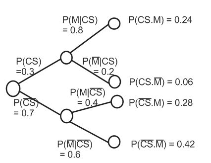
- Notation: Let $ CS $ be the event that the selected student is a computer science major and let $ M $ be the event that the selected student is a male. Therefore, we can define the four events shown below and, summarize the information given problem in the form of a table [2] or in the form of a probability tree
$ CS\equiv \text{CS major; } \overline{CS}\equiv \text{non-major; } M\equiv \text{male; } \overline{M}\equiv \text{female} $
| Total | No. of Male | No. of Female | |
|---|---|---|---|
| No. of CS majors | 0.3 x 200 = 60 | 0.8 x 60 = 48 | 0.2 x 60 = 12 |
| No. of non majors | 0.7 x 200 = 140 | 0.4 x 140 = 56 | 0.6 x 140 = 84 |
| Total | 200 | 104 | 96 |
The elements of the table excluding the legends (or captions) can be considered as a 3x3 matrix. Let (1,1) represent the first cell of the matrix. The content of (1,1) is computed first, followed by content of (1,2) and then (1,3). The same is then done with the second and third rows of the matrix.
The probability tree in Figure 1 is drawn by considering events as sequential. The number of branches in the probability tree depends on the number of events (i.e., how much you know about the problem). The numbers on the branches denote the conditional probabilities. Consider the root node to be at level 0 and thus the leaf nodes to be at level 2. Two events can happen at the root node: $ CS $ or $ \overline{CS} $. Since 30% of students are majors, we get $ \textbf{P}(CS) = 0.3 $ and $ \textbf{P}(\overline{CS}) = 1 - 0.3 = 0.7 $. (P denotes probability). At level 1, two events can happen at each of the nodes, i.e., either a $ M $ or a $ \overline{M} $ can happen. From the problem definition we know that 80% of the CS majors are males, therefore we get, $ \textbf{P}(M\vert CS) = 0.8 $ and $ \textbf{P}(\overline{M}\vert CS) = 1 - 0.8 = 0.2 $. Similarly, we get, $ \textbf{P}(M\vert \overline{CS}) = 0.4 $ and $ \textbf{P}(\overline{M}\vert \overline{CS}) = 0.6 $. It is important to note that the events which can occur at a node are both mutually exhaustive and exclusive. The probability at a leaf node represents the probability of happening of all the events along the path from the root node to that leaf. Note that $ \textbf{P}(CS\cap M) $ and $ \textbf{P}(CS\cdot M) $ are equivalent representations.
- From the table,
$ \textbf{P}(CS) = \frac{\text{No. of CS majors}}{\text{Total no. of Students}} = \frac{60}{200} = 0.3 $
This is nothing but the fraction of the total students who are CS majors. - From the table,
$ \textbf{P}(CS\cap M) = \frac{\text{No. of CS majors who are also males}}{\text{Total no. of Students}} = \frac{48}{200} = 0.24 $
Using the probability tree we can interpret $ (CS\cap M) $ as the occurrence of event $ CS $ followed by the occurrence of event $ M $. Therefore,
$ \textbf{P}(CS\cap M) = \textbf{P}(CS)\times\textbf{P}(M\vert CS) = 0.3\times0.8 = 0.24 \text{ (multiplication rule)} $ - From the table,
$ \textbf{P}(M) = \frac{\text{Total no. males}}{\text{Total no. of Students}} = \frac{104}{200} = 0.52 $
From the probability tree it is clear that the event $ M $ can occur in 2 ways. Therefore we get,$ \textbf{P}(M) = \textbf{P}(M\vert CS)\times \textbf{P}(CS) + \textbf{P}(M\vert \overline{CS})\times \textbf{P}(\overline{CS}) = 0.8\times 0.3 + 0.4\times 0.7 = 0.52\text{ (total probability theorem)} $ - From the table,
$ \textbf{P}(CS\vert M) = \frac{\text{No. of males who are CS majors}}{\text{Total no. of males}} = \frac{48}{104} = 0.4615 $
Now let us compute the same using the probability tree. If you carefully observe the tree it is evident that the computation is not direct. So let us start from the definition of conditional probability, i.e.,$ \textbf{P}(CS\vert M) = \frac{\textbf{P}(CS\cap M)}{\textbf{P}(M)} $
Expanding the numerator using multiplication rule,$ \textbf{P}(CS\vert M) = \frac{\textbf{P}(M\vert CS)\times \textbf{P}(CS)}{\textbf{P}(M)} $
Using total probability theorem in the denominator,$ \textbf{P}(CS\vert M) = \frac{\textbf{P}(M\vert CS)\times \textbf{P}(CS)}{\textbf{P}(M\vert CS)\times \textbf{P}(CS) + \textbf{P}(M\vert \overline{CS})\times \textbf{P}(\overline{CS})}\text{ Eq. (1)} $
Observation:
From part 4. and part 1. we observe that $ \textbf{P}(CS\vert M)>\textbf{P}(CS) $, i.e., $ 0.4615 > 0.3 $. What does this mean? How did the probability that a randomly selected student being a CS major change, when you were informed that the student is a male? Why did it increase?
Explanation:
In part 1. of the problem we only knew the percentage of males and females in the course. So, we computed the probability using just that information. In computing this probability the sample space was the total number of students in the course
In part 4. of the problem we were informed that event $ M $ has occurred, i.e., we got partial information. What did we do with this information? We used it and revised the probability, i.e., our prior belief, in this case $ \textbf{P}(CS) $. $ \textbf{P}(CS) $ is called the prior because that is what we knew about the outcome before being informed about the occurrence of event $ M $. We revised the probability (prior) by changing the sample space from the total number of students to the total number of males in the course. The increase in the prior is justified by the fact that there are more males who are CS majors than females.
Inference:
So, what do we learn from this example?
- We are supposed to revise our beliefs when we get information. Doing this will help us predict the outcome more accurately.
- In this example we computed probabilities using two different methods: constructing a table and, by constructing a probability tree. In practice one could use either of the methods to solve a problem.
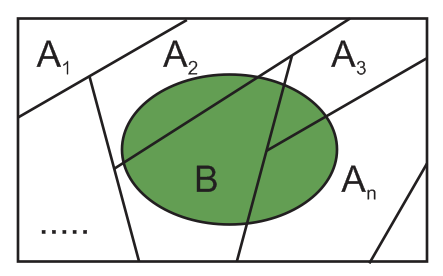
where, $ n $ is the number of events (cardinality of the set $ \{A_{i}\} $) in the sample space and, $ i = 1, 2, ..., n $. Note that the events $ A_{i} $ should be mutually exclusive and exhaustive as shown in the Figure. 2. In Figure. 2 the green colored region corresponds to event $ B $.
Bayes' theorem can be understood better by visualizing the events as sequential as depicted in the probability tree. When additional information is obtained about a subsequent event; it is used to revise the probability of the initial event. The revised probability is called posterior. In other words, we initially have a cause-effect model where we want to predict whether event $ B $ will occur or not, given that event $ A_{i} $ has occurred.
We then move to the inference model where we are told that event $ B $ has occurred and our goal is to infer whether event $ A_{i} $ has occurred or not [3]
In summary, Bayes' Theorem [4] provides us a simple technique to turn information about the probability of different effects (outcomes) from each possible cause, into information about the probable cause given the effect (outcome).
Bayes' Classifier
Bayes' Classifier uses Bayes' theorem (in the form of Bayes' rule) to classify objects into different categories. This technique is widely used in the area of pattern recognition. Let us describe the setting for a classification problem and then briefly outline the procedure.
Problem Setting: Consider a collection of $ N $ objects each with a $ d $ dimensional feature vector $ X $. Let $ X_{k} $ be the feature vector of the $ k^{th} $ object. Feature vector can be thought of as a $ d $-tuple describing the object. The task is to classify the objects into one of the $ C $ categories (classes)
Solution Approach:
Given an object $ k $ with feature vector $ X_{k} $ choose a class $ w_{i} $ such that,Using, Bayes' theorem this can be re-written as,
Since the denominators are the same, we get
Eq. (4) is called Bayes' Rule, where $ \textbf{P}(X_{k}\vert w_{i}) $ and $ \textbf{P}(w_{i}) $ are called the likelihood and prior respectively [5]. Eq. (4), i.e., Bayes' rule is used in the classification problem instead of Eq. (3) because in most real situations it is easier to estimate the likelihood and prior.
References
- D. R. Bellhouse, "The Reverend Thomas Bayes FRS: a Biography to Celebrate the Tercentenary of his Birth," Statistical Science 19, 2004.
- Mario F. Triola, "Bayes' Theorem".
- Dimitri P. Bertsekas, John N. Tsitsiklis, "Introduction to Probability," Second Edition, Athena Scientific, Belmont, Massachusetts, USA, 2008.
- D. S. Sivia, "Data Analysis--A Bayesian Tutorial," Oxford University Press, 1998.
- Mireille Boutin, "ECE662: Statistical Pattern Recognition and Decision Making Processes," Purdue University, Spring 2014.
Questions and comments
If you have any questions, comments, etc. please post them on this page.


