Contents
ECE438 Bonus Point Opportunity
Audio Compression For use in Memory and Computationally Constrained Environments
Christopher Chow, Fall 2016
Introduction and Background
From the earliest wax cylinders made by Thomas Edison [1] to be played on phonographs, to the standard .mp3 file format used ubiquitously today, storing audio has always been an important aspect of the music industry. Even though we are a far cry from only having cassette tapes or vinyl records to store audio, people have always strived to be able to store more songs on smaller and smaller devices. This was no different for my Senior Design project – a remote controlled BB-8 robot which needed to be able to play “realistic astromech droid sounds” [2], with limited processing power as well as limited storage capacity. In our case, the goal was to create an audio compression technique that would:
- Compress audio files down to fit within the flash memory of the microcontroller [3]
- Not be too computationally complex to decode so as to interfere with essential operation of BB-8
- Still sound “okay”; i.e. perceptually not have any huge distortions
Armed with this task, I decided to do what any engineer would do: look for an algorithm that already does what I want it to do. Lossless audio compression methods such as FLAC were dropped almost immediately, as the compression ratios found were much too high (not compressed enough) [4], and while MP3 seemed like the go-to choice, writing an MP3 decoder would likely be more work than the rest of the project itself. Therefore, I decided to try to utilize some concepts from ECE438, such as quantization to create a simple, yet efficient, compression system. A huge portion of audio compression is in the encoding complexity; however, since we will only be playing static data, we don’t have to worry about the encoding complexity of the audio data.
Step 0: Defining Inputs and Outputs
The flow of data is straightforward: from a 16-bit mono PCM .wav file sampled at 48kHz, encode it into some minimized form of data, then be able to decode this data into an array of 8-bit unsigned integers that fits into the microcontroller’s memory to be pushed to the DAC. Therefore, what’s to be stored on the microcontroller is the minimized data for various sounds, so that we can store multiple sound effects (instead of being limited to one 2-second sound effect that fills up all of the flash storage).
Step 1: Finding a minimum sampling rate
While the sounds that BB-8 makes are high pitched, none come close to the maximum 24kHz that a 48kHz sampling rate offers. Additionally, a wonderful feature of the STM32F4xx microcontroller family is that it is able to output audio at arbitrary sampling rates. Therefore, we can specify the sampling rate of a sound effect in its header and then change the DAC output rate to match. Therefore, for each of these sound samples, we can arbitrarily empirically determine a slower sampling rate that doesn't result in a significant loss in quality. I decided that the threshold frequency would be the highest frequency where the magnitude of the FFT of the audio was greater than 2% of the maximum magnitude of the FFT.
MATLAB code for finding a minimum sampling rate
%% Step 1:
%% determine new sampling rate
dataFFT = fftshift(fft(data,512));
dataFFT = dataFFT(257:end);

% determine highest frequency where the magnitude is > 2% of the maximum
% magnitude

% create a vector of booleans corresponding to if the value is greater than
% 2% of the maximum
booleanVector = abs(dataFFT) > max(abs(dataFFT))*0.02;
lastValue = find(booleanVector,1,'last');
thresholdFreq = floor((lastValue/256).*24000);

% resample data to new sampling rate
resampledData = resample(data, thresholdFreq, 24000);
On this sample input, we determine that the threshold frequency is 12750 Hz. So, we can simply use MATLAB's resample function to resample the original data, then prepend the encoded audio file with the sample rate. Of course, the threshold frequency varies for different files; in this case, we have a compression ratio of 53% of the original data size, since the threshold frequency 12750Hz is 53% of 24kHz. Playing the resampled data in MATLAB sounded almost identical to the original sound.
Step 2: Conversion to DAC values
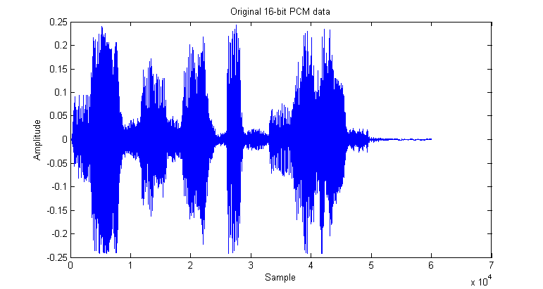
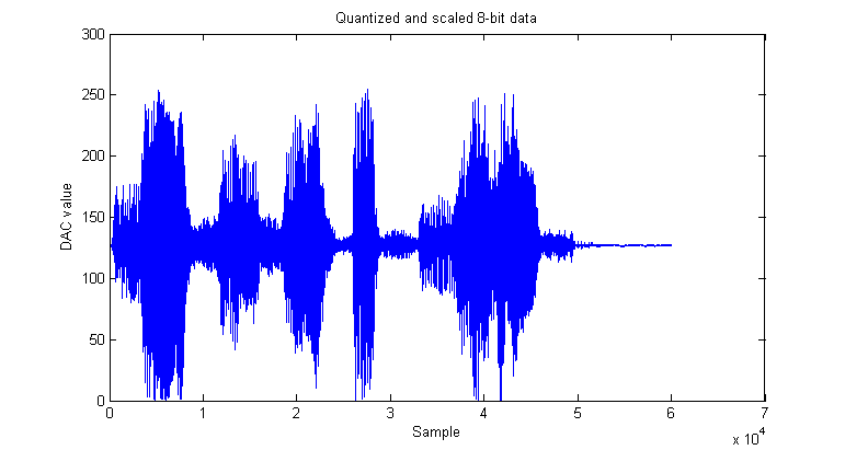
The second step in this process is to quantize the 16-bit data into 8-bits. Of course, since the DAC on our microcontroller only allows for a uniform spacing of output voltage, a max quantizer isn't applicable to this solution. Therefore, we simply uniformly quantize by the following formula: $ Y = \lfloor \frac{X-min(X)}{max(X)}\cdot 255 \rceil $, where Y is the quantized signal and X is the original signal. Below is a plot of our sample input file and its 8-bit quantized version.
Of course, this waveform doesn't look any different, as the original waveform has $ 2^{16} = 65536 $ possible values, while the quantized waveform has $ 2^8 = 256 $ possible values, both quite high. Playing the two sounds side-by-side have almost no perceptible difference in quality.
Step 3: Huffman Coding
The final step in the process is a simple lossless data compression method, Huffman coding [5]. We learned about this in ECE264, and it seems to be the go-to for lossless compression of data. How it works is that it creates a binary tree for each data value and assigns each value to a certain encoded sequence (based on the traversal of the binary tree). Below is the encoding for the data.
%% Step 3: Huffman coding
% create symbols
symbols = unique(quantizedData);
% assign probabilities to each symbol based on a histogram of the data
probabilities = (histc(quantizedData,symbols))./length(quantizedData);
% generate a huffman dictionary
dict = huffmandict(symbols,probabilities);
% Encode the data
encoded = huffmanenco(quantizedData,dict);
The encoded data was 198,407 bits, as compared to the unencoded data, which was 255,216 bits, which was a savings of ~23% from the unencoded data. Since this is a lossless algorithm, the audio data is unaffected. As to the performance of decoding the audio stream, traversing a the Huffman tree and then decoding the data seemed to not affect the performance of the microcontroller significantly.
Conclusions
To summarize: with my compression schemes, I managed to compress the data from its original 120.1kB, down to 63.8kB (resampling), down to 31.9kB (DAC encoding), and finally down to 24.8kB (Huffman coding), for a total of 80% data storage savings! Overall, this is just the beginning for my journey into audio compression for my Senior Design project; there are other lossless and lossy audio compression methods that I haven't tried (such as LPC encoding and as well as drawing from the MP3 compression format), but it's been incredibly useful so far in saving precious flash storage and memory.
References
[1] University of California, Santa Barbara, "The Earliest Wax Cylinders," 2015. [Online]. Available: http://cylinders.library.ucsb.edu/history-wax.php. [Accessed November 2016].
[2] Purdue University, "Digital Systems Senior Design - BB-8 Astromech Droid," August 2016. [Online]. Available: https://engineering.purdue.edu/477grp4/. [Accessed November 2016].
[3] STMicroelectonics, "STM32F405xx, STM32F407xx: ARM Cortex-M4 32b MCU+FPU," September 2016. [Online]. Available: http://www.st.com/content/ccc/resource/technical/document/datasheet/ef/92/76/6d/bb/c2/4f/f7/DM00037051.pdf/files/DM00037051.pdf/jcr:content/translations/en.DM00037051.pdf. [Accessed November 2016].
[4] N. Zachary, "FLAC compression level comparison," 12 June 2014. [Online]. Available: http://z-issue.com/wp/flac-compression-level-comparison/. [Accessed November 2016].
[5] D. Marshall, "Run-Length Encoding (RLE)," 4 Oct 2001 [Online]. Available: https://users.cs.cf.ac.uk/Dave.Marshall/Multimedia/node210.html. [Accessed November 2016].


